7. Forecast predictions in offshore and coastal point all over the world
please contact jtausiahoyal@gmail.com for more information
With this jupyter notebook, forecasts of the waves can be done all over the world just running all the cells below. Data is downloaded from the NOAA website and used for the local predictions. In case the methodology followed wanna be studied in detail, refer to the Forecast class in the repository, and to all the available notebooks as they explain step by step the procedure.
But briefly explained, this notebook download the data, save and plot it and then, reconstruct the predictions using RBF in coastal points using the previously propagated cases with SWAN (refer to the notebooks and the paper in the repo for more information).
# basic imports
import sys
import os
import os.path as op
import datetime

# dev library
sys.path.insert(0, op.join(os.path.abspath('')))

# Forecast module
from forecast import Forecast
date         = datetime.date.today() # today or ex: '20200707'
date         = date.strftime("%Y%m%d")
images_path  = op.join(os.getcwd(), '..', 'images', 'forecast') # save images and GIF
location     = (0, 0) # location to see the forecast

forecast = Forecast(date=date,
                    images_path=images_path,
                    location=location)

print(forecast.forecast)
Pulling the data from:
https://nomads.ncep.noaa.gov/dods/wave/mww3/20201026/multi_1.glo_30mext20201026_00z
The times with forecast go from 2020-10-27 00:00:00 to 2020-11-03 12:00:00
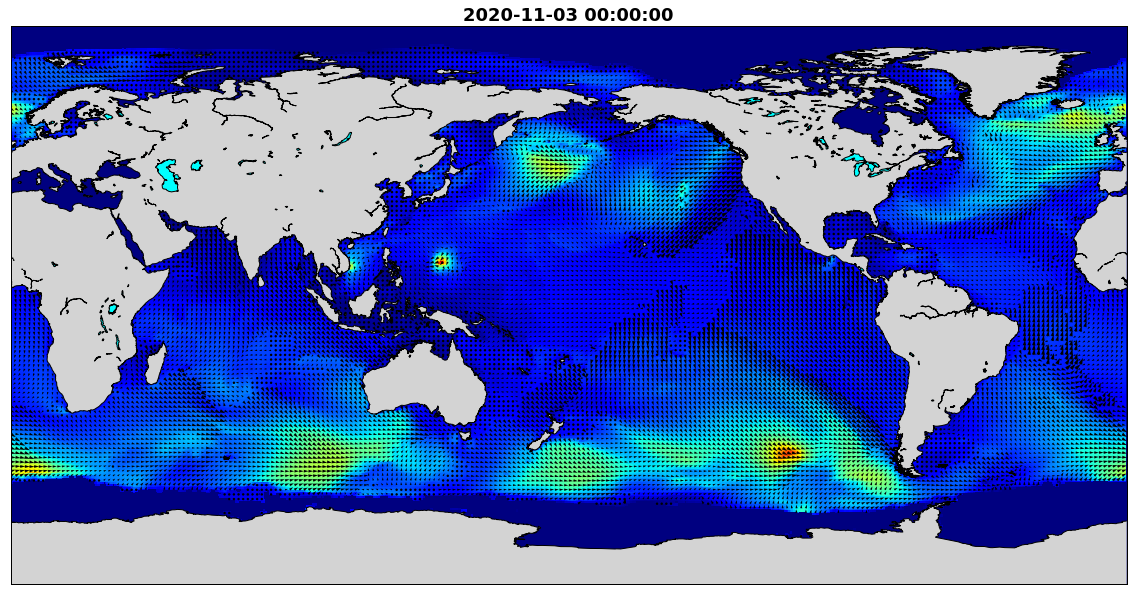
Generating images and GIF in "path"...
Number of images to plot from the total?
TOTAL: 61, To plot:
8
Plotting time: 2020-10-27 00:00:00...
Plotting time: 2020-10-27 21:00:00...
Plotting time: 2020-10-28 18:00:00...
Plotting time: 2020-10-29 15:00:00...
Plotting time: 2020-10-30 12:00:00...
Plotting time: 2020-10-31 09:00:00...
Plotting time: 2020-11-01 06:00:00...
Plotting time: 2020-11-02 03:00:00...
Plotting time: 2020-11-03 00:00:00...
GIF generated and saved!!
<class 'netCDF4._netCDF4.Dataset'>
root group (NETCDF3_CLASSIC data model, file format DAP2):
title: Multi-grid wave model: Global 30 arc-min grid from 00Z26oct2020 downloaded Oct 26 04:24 UTC
Conventions: COARDS
GrADS
dataType: Grid
history: Mon Oct 26 19:05:29 UTC 2020 : imported by GrADS Data Server 2.0
dimensions(sizes): lat(336), lon(720), time(61)
variables(dimensions): float64 time(time), float64 lat(lat), float64 lon(lon), float32 dirpwsfc(time,lat,lon), float32 htsgwsfc(time,lat,lon), float32 perpwsfc(time,lat,lon), float32 swdir_1(time,lat,lon), float32 swdir_2(time,lat,lon), float32 swell_1(time,lat,lon), float32 swell_2(time,lat,lon), float32 swper_1(time,lat,lon), float32 swper_2(time,lat,lon), float32 ugrdsfc(time,lat,lon), float32 vgrdsfc(time,lat,lon), float32 wdirsfc(time,lat,lon), float32 windsfc(time,lat,lon), float32 wvdirsfc(time,lat,lon), float32 wvhgtsfc(time,lat,lon), float32 wvpersfc(time,lat,lon)
groups:
new_location = forecast.select_precise_location()
Move the marker to the exact position:
forecast_nc, forecast_data = forecast.select_region(marker=new_location,
                                                    delta_lon=0.8,
                                                    delta_lat=0.8,
                                                    zoom=8)
New location in [43.96514454266273, -3.6584472656250004]!!

These are the coordinates in the selected region:

[43.5 44.  44.5]
[356.  356.5 357. ]
Saving the data in the shown region...

<xarray.Dataset>
Dimensions:    (lat: 3, lon: 3, time: 61)
Coordinates:
  * time       (time) datetime64[ns] 2020-10-27 ... 2020-11-03T12:00:00
  * lat        (lat) float64 43.5 44.0 44.5
  * lon        (lon) float64 356.0 356.5 357.0
Data variables:
    Hsea       (time, lat, lon) float32 4.02 9.999e+20 ... 9.999e+20 9.999e+20
    Tpsea      (time, lat, lon) float32 14.88 9.999e+20 ... 9.999e+20 9.999e+20
    Dirsea     (time, lat, lon) float32 306.66998 9.999e+20 ... 9.999e+20
    Hswell1    (time, lat, lon) float32 9.999e+20 4.11 4.16 ... 3.25 3.1899998
    Tpswell1   (time, lat, lon) float32 9.999e+20 14.63 ... 14.34 14.389999
    Dirswell1  (time, lat, lon) float32 9.999e+20 306.4 ... 290.5 291.19998
    Hswell2    (time, lat, lon) float32 9.999e+20 9.999e+20 ... 9.999e+20
    Tpswell2   (time, lat, lon) float32 9.999e+20 9.999e+20 ... 9.999e+20
    Dirswell2  (time, lat, lon) float32 9.999e+20 9.999e+20 ... 9.999e+20
    Hs         (time, lat, lon) float32 4.02 4.11 4.16 ... 3.3 3.25 3.1899998
    Tp         (time, lat, lon) float32 14.88 14.63 14.44 ... 14.34 14.389999
    Dir        (time, lat, lon) float32 309.27 307.78 306.93 ... 291.78 292.65
    Uwind      (time, lat, lon) float32 11.65 7.0699997 10.04 ... -4.5 -4.1
    Vwind      (time, lat, lon) float32 -1.64 0.82 -0.16 ... 0.90999997 1.89
    WindSpeed  (time, lat, lon) float32 11.7699995 7.12 10.04 ... 4.5899997 4.52
    DirWind    (time, lat, lon) float32 278.03 263.41 ... 101.409996 114.71

 From the region selected, the closest point will be choosen. Wanna change?

True | False (let box empy) :

 Saving the dataframe with the closest coordinates...

DONE!!
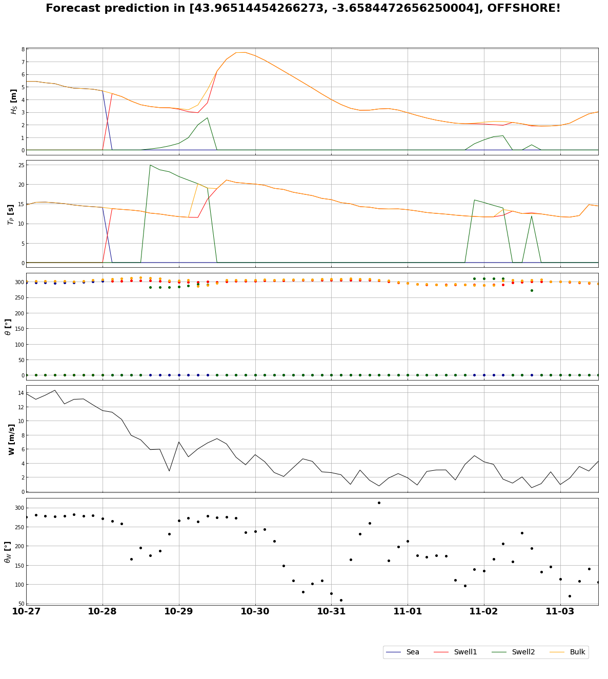
forecast.plot_results(forecast=forecast_data,
                      coast=False)
Important: In the case that NO propagations have been done using SWAN, then the reconstruction in coast cannot be performed, and the notebook ends here.
p_data_swan = op.join(os.getcwd(), '..', 'data', 'projects-swan')

# -------------- EDIT THIS PART --------------------------------------------- #
name = 'SDR'               # used name in the SWAN section
resolution = str(0.0024)   # used resolution in the SWAN section
num_cases = str(300)       # num cases run in SWAN
# --------------------------------------------------------------------------- #

# Example coordinates for the forecast reconstruction:
# Sardinero 43.5, -3.75
# Liencres 43.46, -3.97
# Jeffrey's Bay -34.0 24.98

forecast_recon = forecast.forecast_reconstruction(p_data_swan=p_data_swan,
                                                  forecast_data=forecast_data,
                                                  name=name,
                                                  resolution=resolution,
                                                  num_cases=num_cases)
SUBSETS:

SEA
<class 'pandas.core.frame.DataFrame'>
RangeIndex: 300 entries, 0 to 299
Data columns (total 3 columns):
 #   Column  Non-Null Count  Dtype
---  ------  --------------  -----
 0   hs      300 non-null    float64
 1   per     300 non-null    float64
 2   dir     300 non-null    float64
dtypes: float64(3)
memory usage: 7.2 KB
None
SWELL
<class 'pandas.core.frame.DataFrame'>
RangeIndex: 300 entries, 0 to 299
Data columns (total 3 columns):
 #   Column  Non-Null Count  Dtype
---  ------  --------------  -----
 0   hs      300 non-null    float64
 1   per     300 non-null    float64
 2   dir     300 non-null    float64
dtypes: float64(3)
memory usage: 7.2 KB
None


Select the desired point to reconstruct as it is given in Google Maps:

Latitude location to obtain the forecast reconstruction: 43.46
Longitude location to obtain the forecast reconstruction:
-3.97


TARGETS:

SEA
<class 'pandas.core.frame.DataFrame'>
RangeIndex: 300 entries, 0 to 299
Data columns (total 5 columns):
 #   Column  Non-Null Count  Dtype
---  ------  --------------  -----
 0   hs      300 non-null    float32
 1   per     300 non-null    float32
 2   perM    300 non-null    float32
 3   dir     300 non-null    float32
 4   spr     300 non-null    float32
dtypes: float32(5)
memory usage: 6.0 KB
None
SWELL
<class 'pandas.core.frame.DataFrame'>
RangeIndex: 300 entries, 0 to 299
Data columns (total 5 columns):
 #   Column  Non-Null Count  Dtype
---  ------  --------------  -----
 0   hs      300 non-null    float32
 1   per     300 non-null    float32
 2   perM    300 non-null    float32
 3   dir     300 non-null    float32
 4   spr     300 non-null    float32
dtypes: float32(5)
memory usage: 6.0 KB
None


Forecast in the selected region has the shape:

<class 'pandas.core.frame.DataFrame'>
DatetimeIndex: 61 entries, 2020-10-27 00:00:00 to 2020-11-03 12:00:00
Data columns (total 18 columns):
 #   Column     Non-Null Count  Dtype
---  ------     --------------  -----
 0   Hsea       61 non-null     float32
 1   Tpsea      61 non-null     float32
 2   Dirsea     61 non-null     float32
 3   Hswell1    61 non-null     float32
 4   Tpswell1   61 non-null     float32
 5   Dirswell1  61 non-null     float32
 6   Hswell2    61 non-null     float32
 7   Tpswell2   61 non-null     float32
 8   Dirswell2  61 non-null     float32
 9   Hs         61 non-null     float32
 10  Tp         61 non-null     float32
 11  Dir        61 non-null     float32
 12  Uwind      61 non-null     float32
 13  Vwind      61 non-null     float32
 14  WindSpeed  61 non-null     float32
 15  DirWind    61 non-null     float32
 16  lat        61 non-null     float64
 17  lon        61 non-null     float64
dtypes: float32(16), float64(2)
memory usage: 5.2 KB
None


Performing RFB reconstruction...

ix_scalar: 0,  optimization: 4.98 | interpolation: 0.00
ix_scalar: 1,  optimization: 9.28 | interpolation: 0.00
ix_scalar: 2,  optimization: 6.29 | interpolation: 0.00
ix_scalar: 4,  optimization: 9.53 | interpolation: 0.00
ix_directional: 3,  optimization: 15.76 | interpolation: 0.01
ix_scalar: 0,  optimization: 5.86 | interpolation: 0.01
ix_scalar: 1,  optimization: 10.84 | interpolation: 0.00
ix_scalar: 2,  optimization: 10.85 | interpolation: 0.00
ix_scalar: 4,  optimization: 9.87 | interpolation: 0.00
ix_directional: 3,  optimization: 15.00 | interpolation: 0.01
ix_scalar: 0,  optimization: 5.40 | interpolation: 0.00
ix_scalar: 1,  optimization: 9.99 | interpolation: 0.00
ix_scalar: 2,  optimization: 10.36 | interpolation: 0.00
ix_scalar: 4,  optimization: 11.35 | interpolation: 0.00
ix_directional: 3,  optimization: 14.76 | interpolation: 0.01


Saving the data in path="data/reconstructed/.." ...

                         Hsea      Tpsea      Dirsea   Hswell1   Tpswell1  \
time
2020-10-27 00:00:00  4.440143  14.500299  326.429110  0.000000   0.000000
2020-10-27 03:00:00  4.519804  15.152451  326.552159  0.000000   0.000000
2020-10-27 06:00:00  4.437504  15.209333  326.508203  0.000000   0.000000
2020-10-27 09:00:00  4.358439  15.040860  326.267339  0.000000   0.000000
2020-10-27 12:00:00  4.176344  14.851967  326.207875  0.000000   0.000000
...                       ...        ...         ...       ...        ...
2020-11-03 00:00:00  0.000000   0.000000    0.000000  1.520127  11.622353
2020-11-03 03:00:00  0.000000   0.000000    0.000000  1.649642  11.446942
2020-11-03 06:00:00  0.000000   0.000000    0.000000  1.956715  11.758897
2020-11-03 09:00:00  0.000000   0.000000    0.000000  2.340782  14.719731
2020-11-03 12:00:00  0.000000   0.000000    0.000000  2.485509  14.632953

                      Dirswell1  Hswell2  Tpswell2  Dirswell2        Hs  \
time
2020-10-27 00:00:00    0.000000      0.0       0.0        0.0  4.440143
2020-10-27 03:00:00    0.000000      0.0       0.0        0.0  4.519804
2020-10-27 06:00:00    0.000000      0.0       0.0        0.0  4.437504
2020-10-27 09:00:00    0.000000      0.0       0.0        0.0  4.358439
2020-10-27 12:00:00    0.000000      0.0       0.0        0.0  4.176344
...                         ...      ...       ...        ...       ...
2020-11-03 00:00:00  331.894286      0.0       0.0        0.0  1.520127
2020-11-03 03:00:00  335.861490      0.0       0.0        0.0  1.649642
2020-11-03 06:00:00  333.650244      0.0       0.0        0.0  1.956715
2020-11-03 09:00:00  324.718630      0.0       0.0        0.0  2.340782
2020-11-03 12:00:00  325.268331      0.0       0.0        0.0  2.485509

                            Tp         Dir      Uwind  Vwind  WindSpeed  \
time
2020-10-27 00:00:00  14.500299  326.429110  13.759999  -1.28  13.820000
2020-10-27 03:00:00  15.152451  326.552159  12.820000  -2.31  13.020000
2020-10-27 06:00:00  15.209333  326.508203  13.469999  -1.98  13.610000
2020-10-27 09:00:00  15.040860  326.267339  14.210000  -1.70  14.309999
2020-10-27 12:00:00  14.851967  326.207875  12.240000  -1.78  12.370000
...                        ...         ...        ...    ...        ...
2020-11-03 00:00:00  11.622353  331.894286  -0.890000   0.38   0.960000
2020-11-03 03:00:00  11.446942  335.861490  -1.750000  -0.66   1.870000
2020-11-03 06:00:00  11.758897  333.650244  -3.350000   1.06   3.520000
2020-11-03 09:00:00  14.719731  324.718630  -1.850000   2.20   2.870000
2020-11-03 12:00:00  14.632953  325.268331  -4.110000   1.10   4.260000

                        DirWind
time
2020-10-27 00:00:00  275.329987
2020-10-27 03:00:00  280.229980
2020-10-27 06:00:00  278.369995
2020-10-27 09:00:00  276.809998
2020-10-27 12:00:00  278.279999
...                         ...
2020-11-03 00:00:00  113.049995
2020-11-03 03:00:00   69.290001
2020-11-03 06:00:00  107.610001
2020-11-03 09:00:00  139.970001
2020-11-03 12:00:00  104.949997

[61 rows x 16 columns]

 SAVED!!!
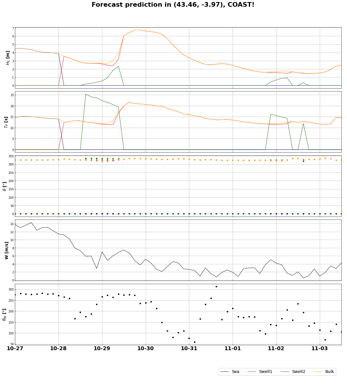
forecast.plot_results(forecast=forecast_recon,
                      coast=True)