4. Final propagation step to wave breaking
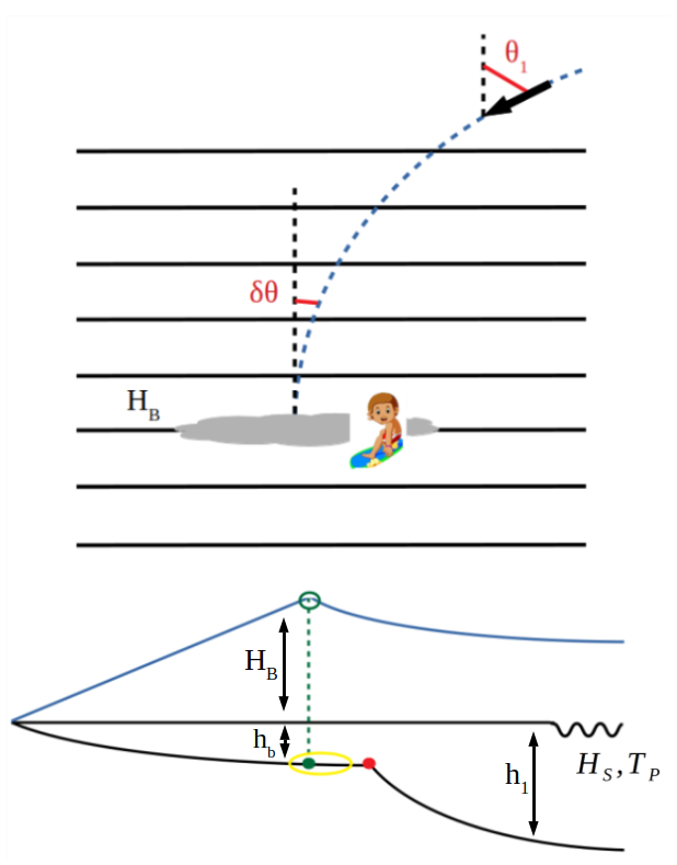
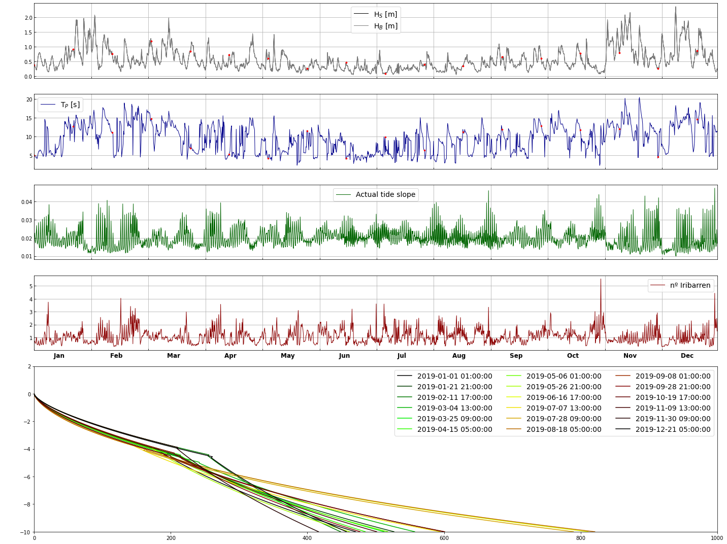
All the data could be propagated to the surfbreak, but we still do not know how waves break, as we do not know their significant wave height at break (\(H_B\)). With this purpose, we proportionate a method to calculate the slope of the beaches, in case we are talking about a beachbreak, so the way waves break and their height can be calculated.
This method uses the law of snell first to propagate waves to the shore and then, knowing the waves that reach the beach, we can estimate the slope that sees the wave when breaking.
This methodology is explained in the figure below (Javier Tausia, 2020), and running the notebook, it will be more clear.
# common
import sys
import os
import os.path as op

# basic
import xarray as xr
import numpy as np
import pandas as pd
from datetime import timedelta as td
from matplotlib import pyplot as plt
from pandas.plotting import register_matplotlib_converters

# dev library
sys.path.insert(0, os.getcwd())

# RBF module
from slopes import Slopes
def wf_calc(A, B):
    d50 = np.exp((0.5 - A)/B)
    wf = 233 * ((d50/1000) ** 1.1)
    print('The values of D50 and wf are, respectively: {}, {}'.format(d50, wf))
    return wf


def index(waves):

    # We first generate the empy lists
    index = []
    index_hb = []
    index_tp = []
    index_spr = []
    index_iri = []
    index_ddir = []
    index_ddirw = []

    # hours, months and years
    waves_month = []
    waves_hour = []
    waves_season = []
    waves_day_moment = []
    waves_year = []

    # We now save the grades
    for i in range(len(waves)):
        if (i%20000)==0:
            print('\n {} waves computed...'.format(i))
        # Compute ihb
        if waves['H_break'][i]<(0.5*1.7):
            ihb = 0
        elif waves['H_break'][i]<(0.7*1.7):
            ihb = 3
        elif waves['H_break'][i]<(1.0*1.7):
            ihb = 7
        elif waves['H_break'][i]<(1.5*1.7):
            ihb = 10
        elif waves['H_break'][i]<(1.8*1.7):
            ihb = 8
        elif waves['H_break'][i]<(2.2*1.7):
            ihb = 5
        elif waves['H_break'][i]<(2.6*1.7):
            ihb = 3
        else:
            ihb = 0
        # Compute itp
        if waves['Tp'][i]<6:
            itp = 0
        elif waves['Tp'][i]<8:
            itp = 3
        elif waves['Tp'][i]<10:
            itp = 5
        elif waves['Tp'][i]<12:
            itp = 7
        elif waves['Tp'][i]<14:
            itp = 9
        else:
            itp = 10
        # Compute ispr
        if waves['Spr'][i]<12:
            ispr = 10
        elif waves['Spr'][i]<15:
            ispr = 9
        elif waves['Spr'][i]<18:
            ispr = 8
        elif waves['Spr'][i]<22:
            ispr = 6
        elif waves['Spr'][i]<26:
            ispr = 4
        else:
            ispr = 2
        # Compute iir
        if waves['Iribarren'][i]<0.3:
            iir = 0
        elif waves['Iribarren'][i]<0.6:
            iir = 3
        elif waves['Iribarren'][i]<0.9:
            iir = 6
        elif waves['Iribarren'][i]<1.2:
            iir = 8
        elif waves['Iribarren'][i]<1.6:
            iir = 10
        elif waves['Iribarren'][i]<1.9:
            iir = 6
        elif waves['Iribarren'][i]<2.2:
            iir = 3
        else:
            iir = 0
        # Compute idd
        if abs(waves['DDir_R'][i])<(20*np.pi/180):
            idd = 0.8
        elif abs(waves['DDir_R'][i])<(30*np.pi/180):
            idd = 1.0
        elif abs(waves['DDir_R'][i])<(50*np.pi/180):
            idd = 1.1
        else:
            idd = 1.2
        # Compute iw
        if abs(waves['DDir_R'][i] - waves['DDirW'][i])<(25*np.pi/180):
            if waves['W'][i]<7:
                iw = 0.8
            elif waves['W'][i]<14:
                iw = 0.5
            else:
                iw = 0.2
        elif abs(waves['DDirW'][i])>(160*np.pi/180):
            if waves['W'][i]<7:
                iw = 1.4
            elif waves['W'][i]<14:
                iw = 1.2
            else:
                iw = 0.9
        elif abs(waves['DDirW'][i])>(130*np.pi/180):
            if waves['W'][i]<7:
                iw = 1.3
            elif waves['W'][i]<14:
                iw = 1.1
            else:
                iw = 0.8
        else:
            if waves['W'][i]<7:
                iw = 1.1
            elif waves['W'][i]<14:
                iw = 0.8
            else:
                iw = 0.6

        index_hb.append(ihb/10)
        index_tp.append(itp/10)
        index_spr.append(ispr/10)
        index_iri.append(iir/10)
        index_ddir.append(idd)
        index_ddirw.append(iw)

        if (int(ihb)==0) or (int(itp)==0):
            index.append(0.1)
        else:
            index.append(((2.6*ihb + 0.7*itp + 0.7*ispr + 0.6*iir) / 50) * iw)

        # time groupings
        month = round(int(str(waves.index.values[i])[5:7]), 0)
        waves_month.append(month)
        if month <= 2:
            waves_season.append('Winter')
        elif month <= 5:
            waves_season.append('Spring')
        elif month <= 8:
            waves_season.append('Summer')
        elif month <= 11:
            waves_season.append('Autumn')
        else:
            waves_season.append('Winter')
        hour = round(int(str(waves.index.values[i])[11:13]), 0)
        waves_hour.append(hour)
        if hour <= 7:
            waves_day_moment.append('night')
        elif hour <= 13:
            waves_day_moment.append('morning')
        elif hour <= 18:
            waves_day_moment.append('afternoon')
        elif hour <= 22:
            waves_day_moment.append('evening')
        else:
            waves_day_moment.append('night')
        waves_year.append(round(int(str(waves.index.values[i])[0:4]), 0))

    waves['Hb_index'] = index_hb
    waves['Tp_index'] = index_tp
    waves['Spr_index'] = index_spr
    waves['Iribarren_index'] = index_iri
    waves['Dir_index'] = index_ddir
    waves['DirW_index'] = index_ddirw
    waves['Index'] = index

    waves['Hour'] = waves_hour
    waves['Day_Moment'] = waves_day_moment
    waves['Month'] = waves_month
    waves['Season'] = waves_season
    waves['Year'] = waves_year

    return waves
# Path to data
p_data = op.join(os.getcwd(), '..', 'data')
# Load the tides
tides = xr.open_dataset(op.join(p_data, 'tides', 'tides_can.nc')).to_dataframe()['ocean_tide'].copy()
# Load the surfbreaks historic
surfbreaks_historic = xr.open_dataset(op.join(p_data, 'reconstructed', 'surfbreaks_reconstructed.nc'))
surfbreaks_historic.beach
<xarray.DataArray 'beach' (beach: 14)>
array(['farolillo', 'bederna', 'oyambre', 'locos', 'valdearenas', 'canallave',
       'madero', 'segunda', 'primera', 'pueblo', 'curva', 'brusco', 'forta',
       'laredo'], dtype=object)
Coordinates:
  * beach    (beach) object 'farolillo' 'bederna' 'oyambre' ... 'forta' 'laredo'
xarray.DataArray
'beach'
- beach: 14
- 'farolillo' 'bederna' 'oyambre' 'locos' ... 'brusco' 'forta' 'laredo'
array(['farolillo', 'bederna', 'oyambre', 'locos', 'valdearenas', 'canallave', 'madero', 'segunda', 'primera', 'pueblo', 'curva', 'brusco', 'forta', 'laredo'], dtype=object) - beach(beach)object'farolillo' 'bederna' ... 'laredo'
array(['farolillo', 'bederna', 'oyambre', 'locos', 'valdearenas', 'canallave',
       'madero', 'segunda', 'primera', 'pueblo', 'curva', 'brusco', 'forta',
       'laredo'], dtype=object)
# Select the surfbreak
name = 'farolillo'
surfbreak = surfbreaks_historic.sel(beach=name).to_dataframe()
delta_angle = 6
wf = 0.030
wf_calculated = wf_calc(1.2738, 0.6157)
print('The wf that will be used is: {}'.format(wf))
reconstructed_depth = 8
farolillo_slope = Slopes(reconstructed_data=surfbreak,
tides=tides,
delta_angle=delta_angle,
wf=wf,
name=name,
reconstructed_depth=reconstructed_depth)
farolillo_slope.perform_propagation()
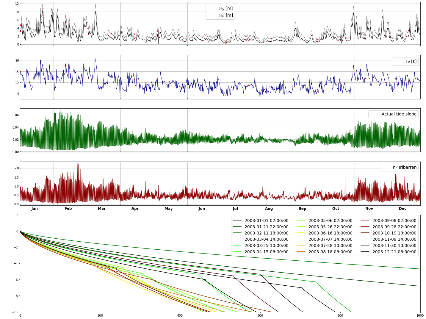
farolillo_slope.moving_profile(year=2003)
farolillo_slope.data = index(farolillo_slope.data)
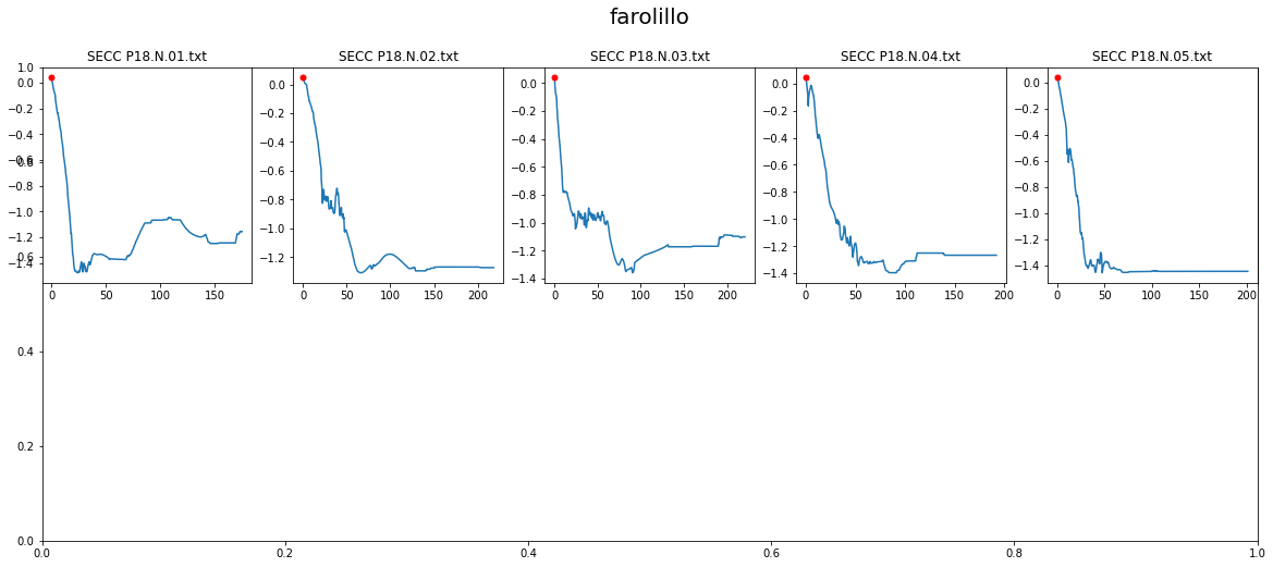
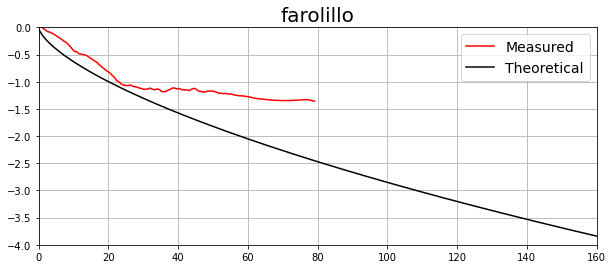
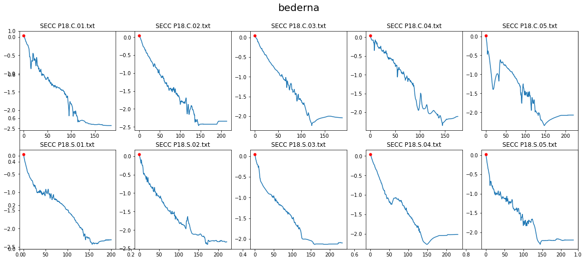
farolillo_slope.validate_profile(root=op.join(p_data, 'profiles'),
omega=farolillo_slope.data.groupby('Month').mean().Omega.iloc[7],
diff_sl=0.5)
farolillo_slope.data['beach'] = name
The values of D50 and wf are, respectively: 0.28456860851215393, 0.02930634178860771
The wf that will be used is: 0.03
Rolling mean and Ω calculated!!
Mean wave direction: -26.66167311837447 º
Mean wind direction: -8.298313693984122 º
Heights asomerament difference: Hb / Hs : 1.6919506218738762
Slopes main object constructed!!
Slopes main object finally constructed!!
<class 'pandas.core.frame.DataFrame'>
DatetimeIndex: 72019 entries, 1979-02-01 02:00:00 to 2020-02-29 20:00:00
Data columns (total 14 columns):
# Column Non-Null Count Dtype
--- ------ -------------- -----
0 Hs 72019 non-null float64
1 Tp 72019 non-null float64
2 Dir 72019 non-null float64
3 Spr 72019 non-null float64
4 W 72019 non-null float64
5 DirW 72019 non-null float64
6 DDir 72019 non-null float64
7 DDirW 72019 non-null float64
8 ocean_tide 72019 non-null float64
9 Omega 72019 non-null float64
10 H_break 72019 non-null float64
11 DDir_R 72019 non-null float64
12 Slope 72019 non-null float64
13 Iribarren 72019 non-null float64
dtypes: float64(14)
memory usage: 8.2 MB
None
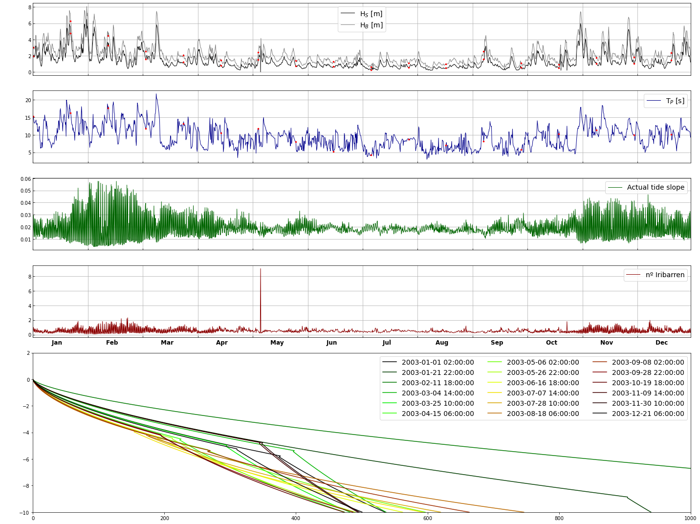
The values of the profiles plotted are:
A B C D Omega
2003-01-01 02:00:00 0.112920 0.002165 0.254160 0.003915 4.853990
2003-01-21 22:00:00 0.096013 0.000759 0.287974 0.001941 5.699339
2003-02-11 18:00:00 0.067146 0.000127 0.345707 0.000586 7.142676
2003-03-04 14:00:00 0.100127 0.000979 0.279746 0.002302 5.493645
2003-03-25 10:00:00 0.113869 0.002296 0.252262 0.004072 4.806550
2003-04-15 06:00:00 0.124927 0.004557 0.230145 0.006444 4.253634
2003-05-06 02:00:00 0.140253 0.011786 0.199494 0.012172 3.487343
2003-05-26 22:00:00 0.129079 0.005895 0.221842 0.007655 4.046055
2003-06-16 18:00:00 0.140050 0.011639 0.199900 0.012070 3.497495
2003-07-07 14:00:00 0.143851 0.014731 0.192298 0.014132 3.307451
2003-07-28 10:00:00 0.145364 0.016180 0.189272 0.015048 3.231811
2003-08-18 06:00:00 0.152730 0.025546 0.174540 0.020428 2.863495
2003-09-08 02:00:00 0.146473 0.017331 0.187055 0.015756 3.176373
2003-09-28 22:00:00 0.130044 0.006259 0.219912 0.007968 3.997805
2003-10-19 18:00:00 0.127807 0.005448 0.224387 0.007262 4.109675
2003-11-09 14:00:00 0.097258 0.000820 0.285484 0.002044 5.637088
2003-11-30 10:00:00 0.096584 0.000786 0.286833 0.001987 5.670821
2003-12-21 06:00:00 0.116734 0.002742 0.246532 0.004586 4.663307
0 waves computed...
20000 waves computed...
40000 waves computed...
60000 waves computed...
# Select the surfbreak
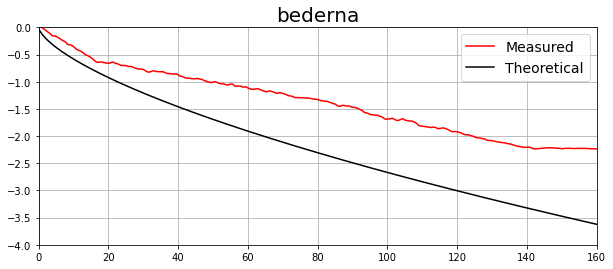
name = 'bederna'
surfbreak = surfbreaks_historic.sel(beach=name).to_dataframe()
delta_angle = 325
wf = 0.035
wf_calculated = wf_calc(1.2897, 0.6585)
print('The wf that will be used is: {}'.format(wf))
reconstructed_depth = 8
bederna_slope = Slopes(reconstructed_data=surfbreak,
tides=tides,
delta_angle=delta_angle,
wf=wf,
name=name,
reconstructed_depth=reconstructed_depth)
bederna_slope.perform_propagation()
bederna_slope.moving_profile(year=2003)
bederna_slope.data = index(bederna_slope.data)
bederna_slope.validate_profile(root=op.join(p_data, 'profiles'),
omega=bederna_slope.data.groupby('Month').mean().Omega.iloc[7],
diff_sl=1.5)
bederna_slope.data['beach'] = name
The values of D50 and wf are, respectively: 0.3014229959588681, 0.031221225164497008
The wf that will be used is: 0.035

 Rolling mean and Ω calculated!!


 Mean wave direction: 4.603694521931204 º


 Mean wind direction: 9.78515820491844 º


 Heights asomerament difference: Hb / Hs : 1.6398351228743209


 Slopes main object constructed!!


 Slopes main object finally constructed!!

<class 'pandas.core.frame.DataFrame'>
DatetimeIndex: 72019 entries, 1979-02-01 02:00:00 to 2020-02-29 20:00:00
Data columns (total 14 columns):
 #   Column      Non-Null Count  Dtype
---  ------      --------------  -----
 0   Hs          72019 non-null  float64
 1   Tp          72019 non-null  float64
 2   Dir         72019 non-null  float64
 3   Spr         72019 non-null  float64
 4   W           72019 non-null  float64
 5   DirW        72019 non-null  float64
 6   DDir        72019 non-null  float64
 7   DDirW       72019 non-null  float64
 8   ocean_tide  72019 non-null  float64
 9   Omega       72019 non-null  float64
 10  H_break     72019 non-null  float64
 11  DDir_R      72019 non-null  float64
 12  Slope       71990 non-null  float64
 13  Iribarren   71990 non-null  float64
dtypes: float64(14)
memory usage: 8.2 MB
None


The values of the profiles plotted are:

                            A         B         C         D     Omega
2003-01-01 02:00:00  0.089398  0.000504  0.301205  0.001475  6.030117
2003-01-21 22:00:00  0.068436  0.000137  0.343128  0.000618  7.078191
2003-02-11 18:00:00  0.047007  0.000036  0.385987  0.000254  8.149669
2003-03-04 14:00:00  0.077318  0.000238  0.325364  0.000893  6.634088
2003-03-25 10:00:00  0.092558  0.000613  0.294884  0.001682  5.872091
2003-04-15 06:00:00  0.119680  0.003292  0.240639  0.005183  4.515987
2003-05-06 02:00:00  0.127292  0.005277  0.225417  0.007108  4.135419
2003-05-26 22:00:00  0.114032  0.002319  0.251936  0.004100  4.798410
2003-06-16 18:00:00  0.124607  0.004468  0.230786  0.006359  4.269641
2003-07-07 14:00:00  0.130185  0.006314  0.219629  0.008015  3.990737
2003-07-28 10:00:00  0.132091  0.007106  0.215818  0.008675  3.895439
2003-08-18 06:00:00  0.141475  0.012714  0.197049  0.012805  3.426227
2003-09-08 02:00:00  0.140785  0.012181  0.198429  0.012444  3.460733
2003-09-28 22:00:00  0.124238  0.004366  0.231525  0.006262  4.288119
2003-10-19 18:00:00  0.122649  0.003957  0.234702  0.005862  4.367559
2003-11-09 14:00:00  0.084930  0.000382  0.310140  0.001225  6.253495
2003-11-30 10:00:00  0.075471  0.000212  0.329058  0.000828  6.726451
2003-12-21 06:00:00  0.101779  0.001085  0.276443  0.002466  5.411067

 0 waves computed...

 20000 waves computed...

 40000 waves computed...

 60000 waves computed...
# Select the surfbreak
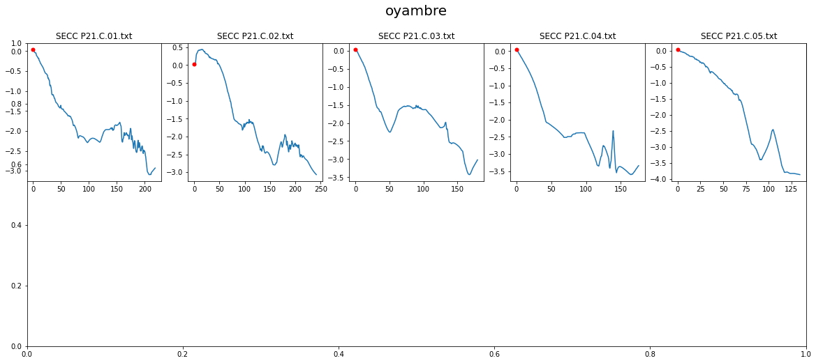
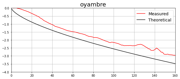
name = 'oyambre'
surfbreak = surfbreaks_historic.sel(beach=name).to_dataframe()
delta_angle = 70
wf = 0.028
wf_calculated = wf_calc(1.2483, 0.5039)
print('The wf that will be used is: {}'.format(wf))
reconstructed_depth = 10
oyambre_slope = Slopes(reconstructed_data=surfbreak,
tides=tides,
delta_angle=delta_angle,
wf=wf,
name=name,
reconstructed_depth=reconstructed_depth)
oyambre_slope.perform_propagation()
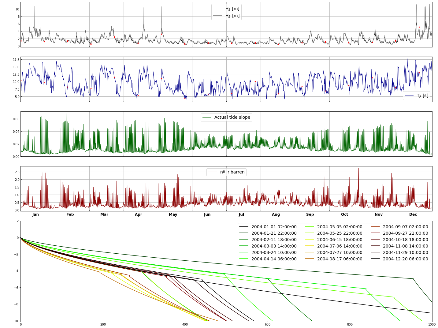
oyambre_slope.moving_profile(year=2004)
oyambre_slope.data = index(oyambre_slope.data)
oyambre_slope.validate_profile(root=op.join(p_data, 'profiles'),
omega=oyambre_slope.data.groupby('Month').mean().Omega.iloc[7],
diff_sl=0.5)
oyambre_slope.data['beach'] = name
The values of D50 and wf are, respectively: 0.2264985199706587, 0.022799631428169796
The wf that will be used is: 0.028

 Rolling mean and Ω calculated!!


 Mean wave direction: -73.41482525749146 º


 Mean wind direction: -31.01464226066187 º


 Heights asomerament difference: Hb / Hs : 1.1295916525429373


 Slopes main object constructed!!


 Slopes main object finally constructed!!

<class 'pandas.core.frame.DataFrame'>
DatetimeIndex: 72019 entries, 1979-02-01 02:00:00 to 2020-02-29 20:00:00
Data columns (total 14 columns):
 #   Column      Non-Null Count  Dtype
---  ------      --------------  -----
 0   Hs          72019 non-null  float64
 1   Tp          72019 non-null  float64
 2   Dir         72019 non-null  float64
 3   Spr         72019 non-null  float64
 4   W           72019 non-null  float64
 5   DirW        72019 non-null  float64
 6   DDir        72019 non-null  float64
 7   DDirW       72019 non-null  float64
 8   ocean_tide  72019 non-null  float64
 9   Omega       72019 non-null  float64
 10  H_break     72019 non-null  float64
 11  DDir_R      72019 non-null  float64
 12  Slope       71873 non-null  float64
 13  Iribarren   71873 non-null  float64
dtypes: float64(14)
memory usage: 8.2 MB
None


The values of the profiles plotted are:

                            A         B         C         D     Omega
2004-01-01 02:00:00  0.087112  0.000437  0.305775  0.001342  6.144377
2004-01-21 22:00:00  0.051242  0.000047  0.377515  0.000303  7.937877
2004-02-11 18:00:00  0.069639  0.000148  0.340723  0.000650  7.018075
2004-03-03 14:00:00  0.093988  0.000669  0.292024  0.001784  5.800602
2004-03-24 10:00:00  0.069459  0.000146  0.341082  0.000645  7.027045
2004-04-14 06:00:00  0.070758  0.000159  0.338484  0.000681  6.962093
2004-05-05 02:00:00  0.076791  0.000230  0.326419  0.000874  6.660466
2004-05-25 22:00:00  0.092178  0.000598  0.295643  0.001655  5.891086
2004-06-15 18:00:00  0.119842  0.003325  0.240317  0.005218  4.507924
2004-07-06 14:00:00  0.113164  0.002198  0.253672  0.003955  4.841796
2004-07-27 10:00:00  0.116768  0.002748  0.246464  0.004593  4.661609
2004-08-17 06:00:00  0.128833  0.005806  0.222334  0.007578  4.058348
2004-09-07 02:00:00  0.112122  0.002060  0.255756  0.003787  4.893903
2004-09-27 22:00:00  0.094122  0.000675  0.291757  0.001794  5.793920
2004-10-18 18:00:00  0.088863  0.000487  0.302273  0.001443  6.056836
2004-11-08 14:00:00  0.092139  0.000597  0.295723  0.001653  5.893072
2004-11-29 10:00:00  0.090884  0.000552  0.298233  0.001569  5.955817
2004-12-20 06:00:00  0.092031  0.000593  0.295939  0.001645  5.898465

 0 waves computed...

 20000 waves computed...

 40000 waves computed...

 60000 waves computed...
# Select the surfbreak
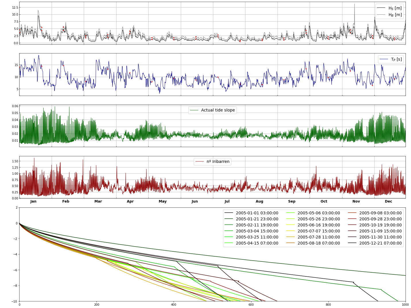
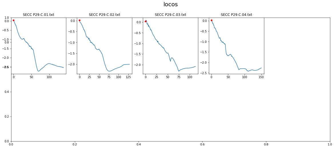
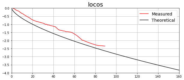
name = 'locos'
surfbreak = surfbreaks_historic.sel(beach=name).to_dataframe()
delta_angle = 295
wf = wf_calc(1.1104, 0.6681)
print('The wf that will be used is: {}'.format(wf))
reconstructed_depth = 5
locos_slope = Slopes(reconstructed_data=surfbreak,
tides=tides,
delta_angle=delta_angle,
wf=wf,
name=name,
reconstructed_depth=reconstructed_depth)
locos_slope.perform_propagation()
locos_slope.moving_profile(year=2005)
locos_slope.data = index(locos_slope.data)
locos_slope.validate_profile(root=op.join(p_data, 'profiles'),
omega=locos_slope.data.groupby('Month').mean().Omega.iloc[7],
diff_sl=0.5)
locos_slope.data['beach'] = name
The values of D50 and wf are, respectively: 0.4010634305424647, 0.042745489201382075
The wf that will be used is: 0.042745489201382075

 Rolling mean and Ω calculated!!


 Mean wave direction: 25.465238302667395 º


 Mean wind direction: 20.764539648217408 º


 Heights asomerament difference: Hb / Hs : 1.437117075964364


 Slopes main object constructed!!


 Slopes main object finally constructed!!

<class 'pandas.core.frame.DataFrame'>
DatetimeIndex: 72019 entries, 1979-02-01 02:00:00 to 2020-02-29 20:00:00
Data columns (total 14 columns):
 #   Column      Non-Null Count  Dtype
---  ------      --------------  -----
 0   Hs          72019 non-null  float64
 1   Tp          72019 non-null  float64
 2   Dir         72019 non-null  float64
 3   Spr         72019 non-null  float64
 4   W           72019 non-null  float64
 5   DirW        72019 non-null  float64
 6   DDir        72019 non-null  float64
 7   DDirW       72019 non-null  float64
 8   ocean_tide  72019 non-null  float64
 9   Omega       72019 non-null  float64
 10  H_break     72019 non-null  float64
 11  DDir_R      72019 non-null  float64
 12  Slope       72019 non-null  float64
 13  Iribarren   72019 non-null  float64
dtypes: float64(14)
memory usage: 8.2 MB
None


The values of the profiles plotted are:

                            A         B         C         D     Omega
2005-01-01 03:00:00  0.083862  0.000357  0.312275  0.001172  6.306885
2005-01-21 23:00:00  0.067415  0.000129  0.345170  0.000592  7.129255
2005-02-11 19:00:00  0.089726  0.000514  0.300548  0.001495  6.013688
2005-03-04 15:00:00  0.104526  0.001286  0.270948  0.002763  5.273689
2005-03-25 11:00:00  0.133113  0.007570  0.213774  0.009050  3.844349
2005-04-15 07:00:00  0.130679  0.006510  0.218641  0.008181  3.966025
2005-05-06 03:00:00  0.111825  0.002023  0.256351  0.003741  4.908763
2005-05-26 23:00:00  0.136775  0.009500  0.206450  0.010536  3.661256
2005-06-16 19:00:00  0.137647  0.010028  0.204706  0.010924  3.617645
2005-07-07 15:00:00  0.136048  0.009081  0.207903  0.010223  3.697580
2005-07-28 11:00:00  0.130001  0.006242  0.219998  0.007954  3.999961
2005-08-18 07:00:00  0.142733  0.013745  0.194533  0.013492  3.363330
2005-09-08 03:00:00  0.134033  0.008015  0.211934  0.009403  3.798354
2005-09-28 23:00:00  0.127229  0.005256  0.225542  0.007090  4.138552
2005-10-19 19:00:00  0.124242  0.004368  0.231516  0.006263  4.287894
2005-11-09 15:00:00  0.111395  0.001969  0.257210  0.003675  4.930256
2005-11-30 11:00:00  0.085916  0.000406  0.308168  0.001277  6.204204
2005-12-21 07:00:00  0.089390  0.000503  0.301221  0.001474  6.030516

 0 waves computed...

 20000 waves computed...

 40000 waves computed...

 60000 waves computed...
# Select the surfbreak
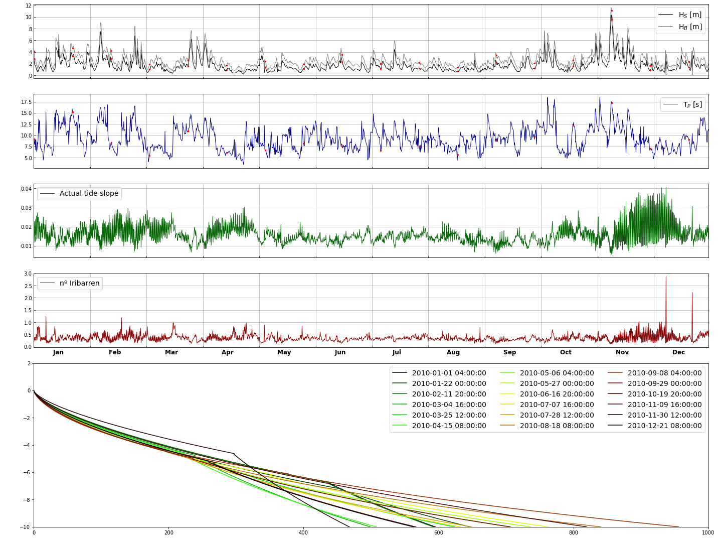
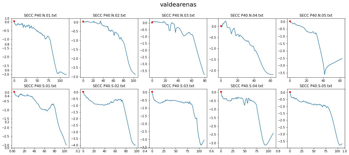
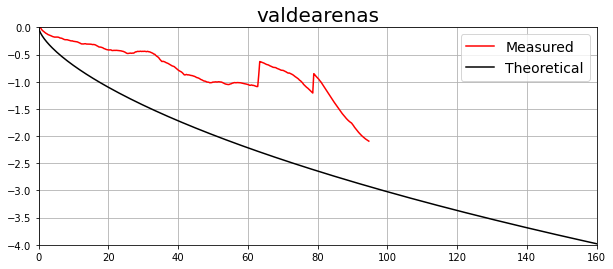
name = 'valdearenas'
surfbreak = surfbreaks_historic.sel(beach=name).to_dataframe()
delta_angle = 340
wf = wf_calc(0.9602, 0.6247)
print('The wf that will be used is: {}'.format(wf))
reconstructed_depth = 8
valdearenas_slope = Slopes(reconstructed_data=surfbreak,
tides=tides,
delta_angle=delta_angle,
wf=wf,
name=name,
reconstructed_depth=reconstructed_depth)
valdearenas_slope.perform_propagation()
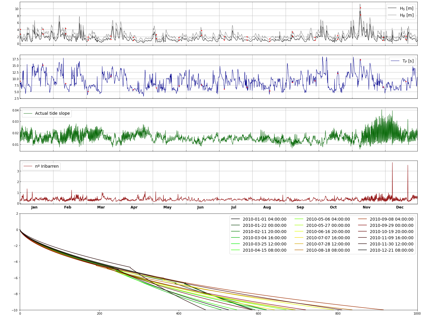
valdearenas_slope.moving_profile(year=2010)
valdearenas_slope.data = index(valdearenas_slope.data)
valdearenas_slope.validate_profile(root=op.join(p_data, 'profiles'),
omega=valdearenas_slope.data.groupby('Month').mean().Omega.iloc[7],
diff_sl=1.5)
valdearenas_slope.data['beach'] = name
The values of D50 and wf are, respectively: 0.4787036282026754, 0.051931314061067546
The wf that will be used is: 0.051931314061067546

 Rolling mean and Ω calculated!!


 Mean wave direction: -8.975274244111828 º


 Mean wind direction: 2.467233362883188 º


 Heights asomerament difference: Hb / Hs : 1.6330347632186633


 Slopes main object constructed!!


 Slopes main object finally constructed!!

<class 'pandas.core.frame.DataFrame'>
DatetimeIndex: 72019 entries, 1979-02-01 02:00:00 to 2020-02-29 20:00:00
Data columns (total 14 columns):
 #   Column      Non-Null Count  Dtype
---  ------      --------------  -----
 0   Hs          72019 non-null  float64
 1   Tp          72019 non-null  float64
 2   Dir         72019 non-null  float64
 3   Spr         72019 non-null  float64
 4   W           72019 non-null  float64
 5   DirW        72019 non-null  float64
 6   DDir        72019 non-null  float64
 7   DDirW       72019 non-null  float64
 8   ocean_tide  72019 non-null  float64
 9   Omega       72019 non-null  float64
 10  H_break     72019 non-null  float64
 11  DDir_R      72019 non-null  float64
 12  Slope       72019 non-null  float64
 13  Iribarren   72019 non-null  float64
dtypes: float64(14)
memory usage: 8.2 MB
None


The values of the profiles plotted are:

                            A         B         C         D     Omega
2010-01-01 04:00:00  0.122626  0.003951  0.234748  0.005857  4.368698
2010-01-22 00:00:00  0.135601  0.008833  0.208798  0.010035  3.719946
2010-02-11 20:00:00  0.122388  0.003893  0.235224  0.005799  4.380606
2010-03-04 16:00:00  0.128429  0.005662  0.223143  0.007452  4.078564
2010-03-25 12:00:00  0.142843  0.013839  0.194314  0.013553  3.357839
2010-04-15 08:00:00  0.131460  0.006833  0.217080  0.008451  3.926988
2010-05-06 04:00:00  0.149519  0.020935  0.180961  0.017880  3.024026
2010-05-27 00:00:00  0.151618  0.023844  0.176764  0.019507  2.919088
2010-06-16 20:00:00  0.151592  0.023806  0.176816  0.019486  2.920393
2010-07-07 16:00:00  0.144790  0.015615  0.190419  0.014694  3.260479
2010-07-28 12:00:00  0.146194  0.017035  0.187612  0.015575  3.190304
2010-08-18 08:00:00  0.156596  0.032465  0.166809  0.023983  2.670219
2010-09-08 04:00:00  0.159764  0.039512  0.160472  0.027353  2.511790
2010-09-29 00:00:00  0.149721  0.021198  0.180558  0.018030  3.013951
2010-10-19 20:00:00  0.136887  0.009566  0.206226  0.010585  3.655660
2010-11-09 16:00:00  0.124922  0.004556  0.230157  0.006442  4.253917
2010-11-30 12:00:00  0.104905  0.001317  0.270191  0.002807  5.254764
2010-12-21 08:00:00  0.136646  0.009424  0.206709  0.010479  3.667721

 0 waves computed...

 20000 waves computed...

 40000 waves computed...

 60000 waves computed...
# Select the surfbreak
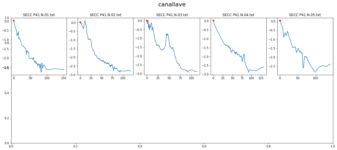
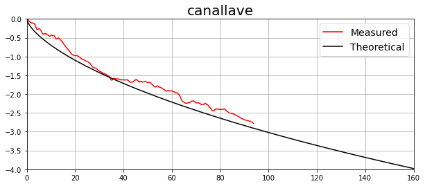
name = 'canallave'
surfbreak = surfbreaks_historic.sel(beach=name).to_dataframe()
delta_angle = 350
wf = wf_calc(0.9852, 0.6154)
print('The wf that will be used is: {}'.format(wf))
reconstructed_depth = 10
canallave_slope = Slopes(reconstructed_data=surfbreak,
tides=tides,
delta_angle=delta_angle,
wf=wf,
name=name,
reconstructed_depth=reconstructed_depth)
canallave_slope.perform_propagation()
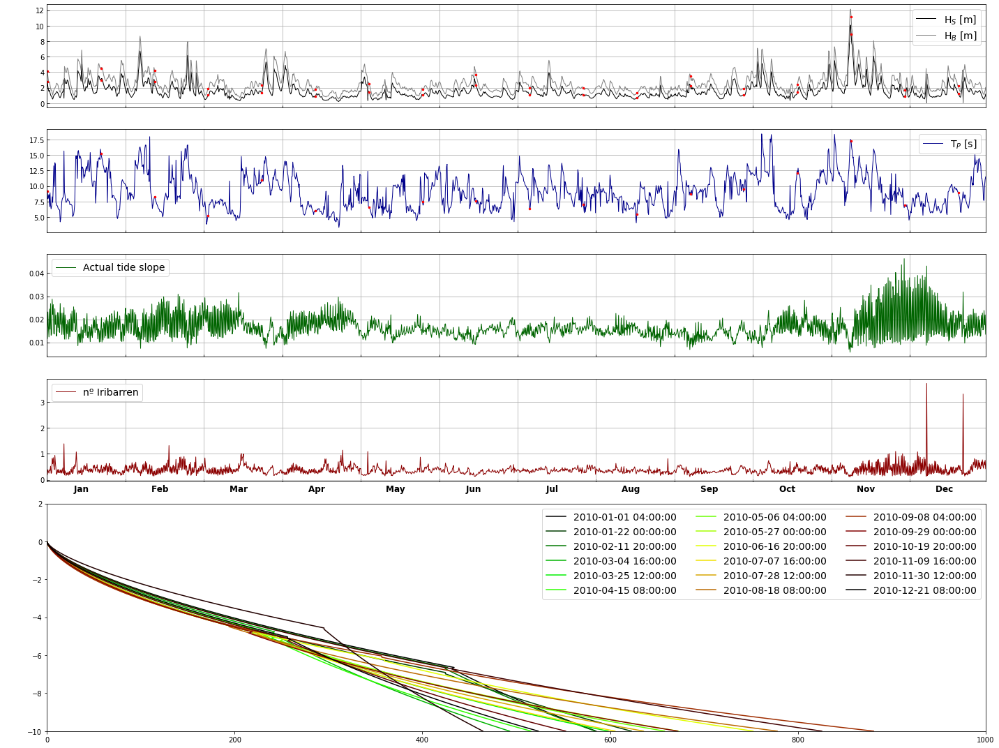
canallave_slope.moving_profile(year=2010)
canallave_slope.data = index(canallave_slope.data)
canallave_slope.validate_profile(root=op.join(p_data, 'profiles'),
omega=canallave_slope.data.groupby('Month').mean().Omega.iloc[7],
diff_sl=1.5)
canallave_slope.data['beach'] = name
The values of D50 and wf are, respectively: 0.4545577597672397, 0.04905732967163039
The wf that will be used is: 0.04905732967163039

 Rolling mean and Ω calculated!!


 Mean wave direction: -27.102964299627416 º


 Mean wind direction: -2.2949881203226643 º


 Heights asomerament difference: Hb / Hs : 1.6833531174171443


 Slopes main object constructed!!


 Slopes main object finally constructed!!

<class 'pandas.core.frame.DataFrame'>
DatetimeIndex: 72019 entries, 1979-02-01 02:00:00 to 2020-02-29 20:00:00
Data columns (total 14 columns):
 #   Column      Non-Null Count  Dtype
---  ------      --------------  -----
 0   Hs          72019 non-null  float64
 1   Tp          72019 non-null  float64
 2   Dir         72019 non-null  float64
 3   Spr         72019 non-null  float64
 4   W           72019 non-null  float64
 5   DirW        72019 non-null  float64
 6   DDir        72019 non-null  float64
 7   DDirW       72019 non-null  float64
 8   ocean_tide  72019 non-null  float64
 9   Omega       72019 non-null  float64
 10  H_break     72019 non-null  float64
 11  DDir_R      72019 non-null  float64
 12  Slope       72019 non-null  float64
 13  Iribarren   72019 non-null  float64
dtypes: float64(14)
memory usage: 8.2 MB
None


The values of the profiles plotted are:

                            A         B         C         D     Omega
2010-01-01 04:00:00  0.125007  0.004580  0.229986  0.006465  4.249651
2010-01-22 00:00:00  0.136861  0.009551  0.206278  0.010574  3.656953
2010-02-11 20:00:00  0.127676  0.005404  0.224649  0.007222  4.116221
2010-03-04 16:00:00  0.130211  0.006324  0.219578  0.008024  3.989451
2010-03-25 12:00:00  0.143327  0.014260  0.193347  0.013828  3.333663
2010-04-15 08:00:00  0.136592  0.009393  0.206816  0.010456  3.670390
2010-05-06 04:00:00  0.146953  0.017855  0.186094  0.016073  3.152359
2010-05-27 00:00:00  0.148901  0.020147  0.182198  0.017427  3.054960
2010-06-16 20:00:00  0.152936  0.025874  0.174129  0.020603  2.853215
2010-07-07 16:00:00  0.145556  0.016374  0.188887  0.015168  3.222180
2010-07-28 12:00:00  0.149128  0.020433  0.181743  0.017592  3.043586
2010-08-18 08:00:00  0.156612  0.032498  0.166775  0.024000  2.669385
2010-09-08 04:00:00  0.158363  0.036223  0.163275  0.025808  2.581867
2010-09-29 00:00:00  0.150734  0.022572  0.178533  0.018804  2.963313
2010-10-19 20:00:00  0.139571  0.011298  0.200859  0.011832  3.521470
2010-11-09 16:00:00  0.128376  0.005644  0.223248  0.007435  4.081194
2010-11-30 12:00:00  0.111883  0.002030  0.256234  0.003750  4.905853
2010-12-21 08:00:00  0.132263  0.007182  0.215474  0.008737  3.886852

 0 waves computed...

 20000 waves computed...

 40000 waves computed...

 60000 waves computed...
# Select the surfbreak
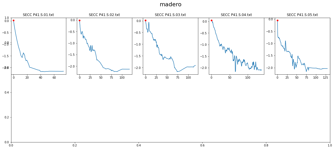
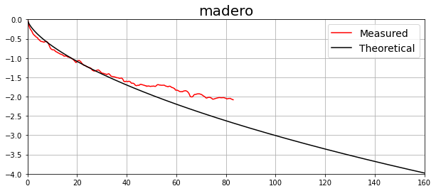
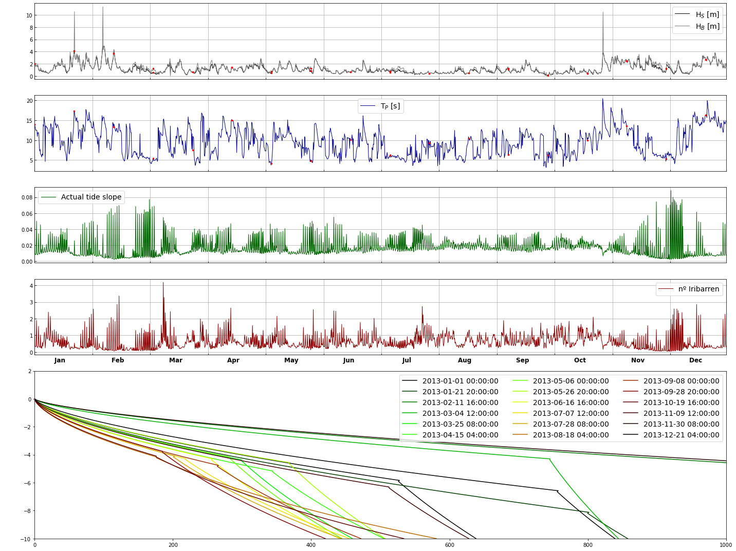
name = 'madero'
surfbreak = surfbreaks_historic.sel(beach=name).to_dataframe()
delta_angle = 350
wf = 0.047
wf_calculated = wf_calc(1.1839, 0.6660)
print('The wf that will be used is: {}'.format(wf))
reconstructed_depth = 10
madero_slope = Slopes(reconstructed_data=surfbreak,
tides=tides,
delta_angle=delta_angle,
wf=wf,
name=name,
reconstructed_depth=reconstructed_depth)
madero_slope.perform_propagation()
madero_slope.moving_profile(year=2010)
madero_slope.data = index(madero_slope.data)
madero_slope.validate_profile(root=op.join(p_data, 'profiles'),
omega=madero_slope.data.groupby('Month').mean().Omega.iloc[7],
diff_sl=0.8)
madero_slope.data['beach'] = name
The values of D50 and wf are, respectively: 0.3581236801815413, 0.03773916297995551
The wf that will be used is: 0.047

 Rolling mean and Ω calculated!!


 Mean wave direction: -25.106096208720885 º


 Mean wind direction: -2.2949881203226643 º


 Heights asomerament difference: Hb / Hs : 1.6907088860620965


 Slopes main object constructed!!


 Slopes main object finally constructed!!

<class 'pandas.core.frame.DataFrame'>
DatetimeIndex: 72019 entries, 1979-02-01 02:00:00 to 2020-02-29 20:00:00
Data columns (total 14 columns):
 #   Column      Non-Null Count  Dtype
---  ------      --------------  -----
 0   Hs          72019 non-null  float64
 1   Tp          72019 non-null  float64
 2   Dir         72019 non-null  float64
 3   Spr         72019 non-null  float64
 4   W           72019 non-null  float64
 5   DirW        72019 non-null  float64
 6   DDir        72019 non-null  float64
 7   DDirW       72019 non-null  float64
 8   ocean_tide  72019 non-null  float64
 9   Omega       72019 non-null  float64
 10  H_break     72019 non-null  float64
 11  DDir_R      72019 non-null  float64
 12  Slope       72019 non-null  float64
 13  Iribarren   72019 non-null  float64
dtypes: float64(14)
memory usage: 8.2 MB
None


The values of the profiles plotted are:

                            A         B         C         D     Omega
2010-01-01 04:00:00  0.120485  0.003460  0.239030  0.005359  4.475759
2010-01-22 00:00:00  0.133903  0.007950  0.212194  0.009352  3.804844
2010-02-11 20:00:00  0.122325  0.003878  0.235351  0.005784  4.383772
2010-03-04 16:00:00  0.126877  0.005143  0.226246  0.006987  4.156147
2010-03-25 12:00:00  0.141653  0.012855  0.196694  0.012900  3.417343
2010-04-15 08:00:00  0.132431  0.007257  0.215137  0.008798  3.878433
2010-05-06 04:00:00  0.146467  0.017326  0.187066  0.015753  3.176641
2010-05-27 00:00:00  0.147943  0.018986  0.184114  0.016748  3.102854
2010-06-16 20:00:00  0.150505  0.022254  0.178990  0.018627  2.974742
2010-07-07 16:00:00  0.142602  0.013634  0.194795  0.013418  3.369883
2010-07-28 12:00:00  0.145157  0.015974  0.189685  0.014919  3.242127
2010-08-18 08:00:00  0.153997  0.027634  0.172006  0.021531  2.800146
2010-09-08 04:00:00  0.157049  0.033390  0.165902  0.024439  2.647545
2010-09-29 00:00:00  0.148136  0.019215  0.183727  0.016883  3.093179
2010-10-19 20:00:00  0.135595  0.008829  0.208811  0.010032  3.720272
2010-11-09 16:00:00  0.123322  0.004125  0.233357  0.006028  4.333920
2010-11-30 12:00:00  0.103756  0.001226  0.272487  0.002677  5.312185
2010-12-21 08:00:00  0.130846  0.006578  0.218307  0.008238  3.957678

 0 waves computed...

 20000 waves computed...

 40000 waves computed...

 60000 waves computed...
# Select the surfbreak
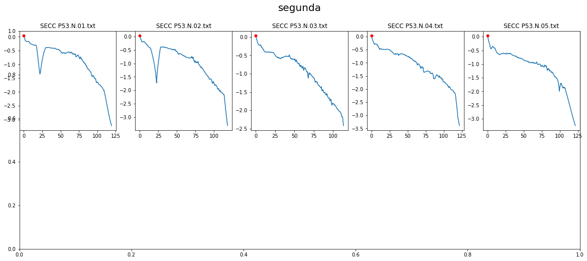
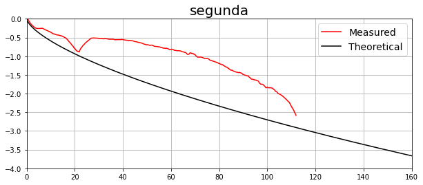
name = 'segunda'
surfbreak = surfbreaks_historic.sel(beach=name).to_dataframe()
delta_angle = 75
wf = 0.022
wf_calulated = wf_calc(1.0988, 0.5929)
print('The wf that will be used is: {}'.format(wf))
reconstructed_depth = 10
segunda_slope = Slopes(reconstructed_data=surfbreak,
tides=tides,
delta_angle=delta_angle,
wf=wf,
name=name,
reconstructed_depth=reconstructed_depth)
segunda_slope.perform_propagation()
segunda_slope.moving_profile(year=2013)
segunda_slope.data = index(segunda_slope.data)
segunda_slope.validate_profile(root=op.join(p_data, 'profiles'),
omega=segunda_slope.data.groupby('Month').mean().Omega.iloc[7],
diff_sl=1.0)
segunda_slope.data['beach'] = name
The values of D50 and wf are, respectively: 0.36423679473213266, 0.038448386404837304
The wf that will be used is: 0.022

 Rolling mean and Ω calculated!!


 Mean wave direction: -76.70821460688457 º


 Mean wind direction: -31.46026913129706 º


 Heights asomerament difference: Hb / Hs : 1.120889300470879


 Slopes main object constructed!!


 Slopes main object finally constructed!!

<class 'pandas.core.frame.DataFrame'>
DatetimeIndex: 72019 entries, 1979-02-01 02:00:00 to 2020-02-29 20:00:00
Data columns (total 14 columns):
 #   Column      Non-Null Count  Dtype
---  ------      --------------  -----
 0   Hs          72019 non-null  float64
 1   Tp          72019 non-null  float64
 2   Dir         72019 non-null  float64
 3   Spr         72019 non-null  float64
 4   W           72019 non-null  float64
 5   DirW        72019 non-null  float64
 6   DDir        72019 non-null  float64
 7   DDirW       72019 non-null  float64
 8   ocean_tide  72019 non-null  float64
 9   Omega       72019 non-null  float64
 10  H_break     72019 non-null  float64
 11  DDir_R      72019 non-null  float64
 12  Slope       72019 non-null  float64
 13  Iribarren   72019 non-null  float64
dtypes: float64(14)
memory usage: 8.2 MB
None


The values of the profiles plotted are:

                            A         B         C         D     Omega
2013-01-01 00:00:00  0.089860  0.000518  0.300279  0.001504  6.006979
2013-01-21 20:00:00  0.095151  0.000719  0.289698  0.001873  5.742447
2013-02-11 16:00:00  0.045701  0.000034  0.388598  0.000241  8.214954
2013-03-04 12:00:00  0.052279  0.000050  0.375442  0.000316  7.886053
2013-03-25 08:00:00  0.098028  0.000860  0.283944  0.002110  5.598598
2013-04-15 04:00:00  0.106385  0.001444  0.267230  0.002985  5.180760
2013-05-06 00:00:00  0.097257  0.000820  0.285487  0.002044  5.637167
2013-05-26 20:00:00  0.089153  0.000496  0.301693  0.001460  6.042336
2013-06-16 16:00:00  0.107085  0.001508  0.265830  0.003073  5.145753
2013-07-07 12:00:00  0.120836  0.003536  0.238328  0.005437  4.458205
2013-07-28 08:00:00  0.120967  0.003565  0.238067  0.005467  4.451669
2013-08-18 04:00:00  0.142079  0.013199  0.195842  0.013130  3.396053
2013-09-08 00:00:00  0.117472  0.002870  0.245056  0.004729  4.626408
2013-09-28 20:00:00  0.117354  0.002849  0.245293  0.004706  4.632323
2013-10-19 16:00:00  0.137517  0.009947  0.204965  0.010866  3.624133
2013-11-09 12:00:00  0.099490  0.000941  0.281020  0.002242  5.525489
2013-11-30 08:00:00  0.044355  0.000031  0.391291  0.000227  8.282264
2013-12-21 04:00:00  0.079418  0.000271  0.321165  0.000975  6.529124

 0 waves computed...

 20000 waves computed...

 40000 waves computed...

 60000 waves computed...
# Select the surfbreak
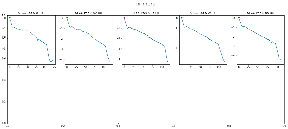
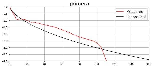
name = 'primera'
surfbreak = surfbreaks_historic.sel(beach=name).to_dataframe()
delta_angle = 70
wf = 0.024
wf_calculated = wf_calc(1.1364, 0.6160)
print('The wf that will be used is: {}'.format(wf))
reconstructed_depth = 8
primera_slope = Slopes(reconstructed_data=surfbreak,
tides=tides,
delta_angle=delta_angle,
wf=wf,
name=name,
reconstructed_depth=reconstructed_depth)
primera_slope.perform_propagation()
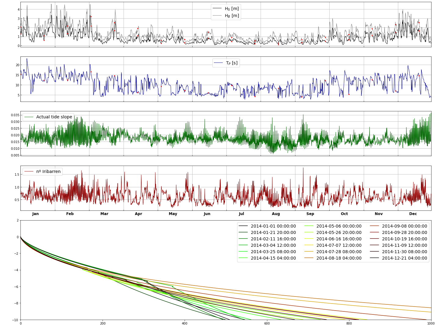
primera_slope.moving_profile(year=2014)
primera_slope.data = index(primera_slope.data)
primera_slope.validate_profile(root=op.join(p_data, 'profiles'),
omega=primera_slope.data.groupby('Month').mean().Omega.iloc[7],
diff_sl=1.5)
primera_slope.data['beach'] = name
The values of D50 and wf are, respectively: 0.3558959439550598, 0.03748100810819603
The wf that will be used is: 0.024

 Rolling mean and Ω calculated!!


 Mean wave direction: -33.93958535504187 º


 Mean wind direction: -31.01464226066187 º


 Heights asomerament difference: Hb / Hs : 1.8970812974240645


 Slopes main object constructed!!


 Slopes main object finally constructed!!

<class 'pandas.core.frame.DataFrame'>
DatetimeIndex: 72019 entries, 1979-02-01 02:00:00 to 2020-02-29 20:00:00
Data columns (total 14 columns):
 #   Column      Non-Null Count  Dtype
---  ------      --------------  -----
 0   Hs          72019 non-null  float64
 1   Tp          72019 non-null  float64
 2   Dir         72019 non-null  float64
 3   Spr         72019 non-null  float64
 4   W           72019 non-null  float64
 5   DirW        72019 non-null  float64
 6   DDir        72019 non-null  float64
 7   DDirW       72019 non-null  float64
 8   ocean_tide  72019 non-null  float64
 9   Omega       72019 non-null  float64
 10  H_break     72019 non-null  float64
 11  DDir_R      72019 non-null  float64
 12  Slope       72019 non-null  float64
 13  Iribarren   72019 non-null  float64
dtypes: float64(14)
memory usage: 8.2 MB
None


The values of the profiles plotted are:

                            A         B         C         D     Omega
2014-01-01 00:00:00  0.134871  0.008442  0.210258  0.009735  3.756461
2014-01-21 20:00:00  0.132496  0.007286  0.215009  0.008822  3.875221
2014-02-11 16:00:00  0.117328  0.002845  0.245345  0.004701  4.633625
2014-03-04 12:00:00  0.119054  0.003166  0.241892  0.005050  4.547308
2014-03-25 08:00:00  0.134796  0.008403  0.210409  0.009705  3.760221
2014-04-15 04:00:00  0.145040  0.015858  0.189920  0.014847  3.248006
2014-05-06 00:00:00  0.152356  0.024961  0.175288  0.020114  2.882198
2014-05-26 20:00:00  0.150069  0.021661  0.179862  0.018293  2.996546
2014-06-16 16:00:00  0.156880  0.033041  0.166241  0.024267  2.656024
2014-07-07 12:00:00  0.154936  0.029290  0.170128  0.022387  2.753212
2014-07-28 08:00:00  0.167682  0.064555  0.144635  0.037995  2.115884
2014-08-18 04:00:00  0.171126  0.079920  0.137748  0.043831  1.943709
2014-09-08 00:00:00  0.161622  0.044335  0.156756  0.029545  2.418911
2014-09-28 20:00:00  0.156087  0.031458  0.167825  0.023482  2.695632
2014-10-19 16:00:00  0.155749  0.030804  0.168503  0.023155  2.712565
2014-11-09 12:00:00  0.152279  0.024841  0.175442  0.020049  2.886058
2014-11-30 08:00:00  0.146758  0.017640  0.186485  0.015944  3.162119
2014-12-21 04:00:00  0.120761  0.003520  0.238478  0.005421  4.461961

 0 waves computed...

 20000 waves computed...

 40000 waves computed...

 60000 waves computed...
# Select the surfbreak
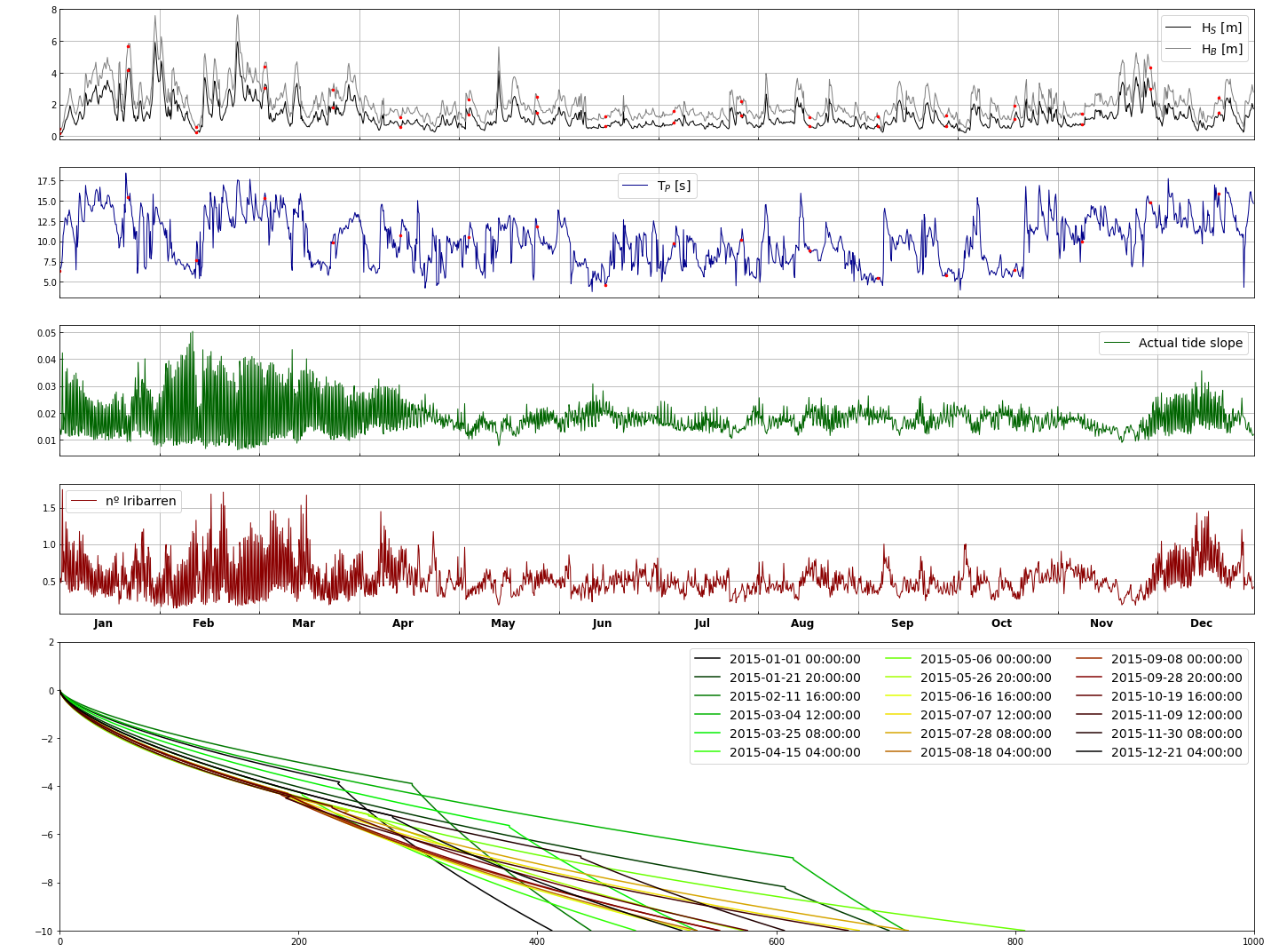
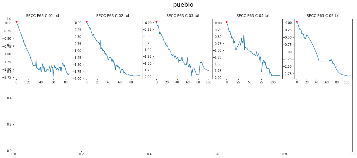
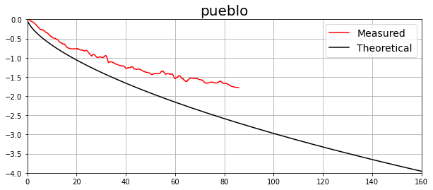
name = 'pueblo'
surfbreak = surfbreaks_historic.sel(beach=name).to_dataframe()
delta_angle = 355
wf = 0.032
wf_calculated = wf_calc(1.2887, 0.6627)
print('The wf that will be used is: {}'.format(wf))
reconstructed_depth = 8
pueblo_slope = Slopes(reconstructed_data=surfbreak,
tides=tides,
delta_angle=delta_angle,
wf=wf,
name=name,
reconstructed_depth=reconstructed_depth)
pueblo_slope.perform_propagation()
pueblo_slope.moving_profile(year=2015)
pueblo_slope.data = index(pueblo_slope.data)
pueblo_slope.validate_profile(root=op.join(p_data, 'profiles'),
omega=pueblo_slope.data.groupby('Month').mean().Omega.iloc[7],
diff_sl=1.6)
pueblo_slope.data['beach'] = name
The values of D50 and wf are, respectively: 0.3041813281790857, 0.03153564572726523
The wf that will be used is: 0.032

 Rolling mean and Ω calculated!!


 Mean wave direction: -12.683316823428534 º


 Mean wind direction: -4.301971825011723 º


 Heights asomerament difference: Hb / Hs : 1.8018422576128574


 Slopes main object constructed!!


 Slopes main object finally constructed!!

<class 'pandas.core.frame.DataFrame'>
DatetimeIndex: 72019 entries, 1979-02-01 02:00:00 to 2020-02-29 20:00:00
Data columns (total 14 columns):
 #   Column      Non-Null Count  Dtype
---  ------      --------------  -----
 0   Hs          72019 non-null  float64
 1   Tp          72019 non-null  float64
 2   Dir         72019 non-null  float64
 3   Spr         72019 non-null  float64
 4   W           72019 non-null  float64
 5   DirW        72019 non-null  float64
 6   DDir        72019 non-null  float64
 7   DDirW       72019 non-null  float64
 8   ocean_tide  72019 non-null  float64
 9   Omega       72019 non-null  float64
 10  H_break     72019 non-null  float64
 11  DDir_R      72019 non-null  float64
 12  Slope       72019 non-null  float64
 13  Iribarren   72019 non-null  float64
dtypes: float64(14)
memory usage: 8.2 MB
None


The values of the profiles plotted are:

                            A         B         C         D     Omega
2015-01-01 00:00:00  0.101167  0.001045  0.277665  0.002404  5.441625
2015-01-21 20:00:00  0.120115  0.003382  0.239769  0.005277  4.494235
2015-02-11 16:00:00  0.088018  0.000462  0.303965  0.001393  6.099114
2015-03-04 12:00:00  0.097590  0.000837  0.284819  0.002072  5.620484
2015-03-25 08:00:00  0.109832  0.001787  0.260337  0.003444  5.008424
2015-04-15 04:00:00  0.128527  0.005697  0.222947  0.007482  4.073669
2015-05-06 00:00:00  0.154751  0.028956  0.170498  0.022216  2.762450
2015-05-26 20:00:00  0.137588  0.009991  0.204823  0.010898  3.620584
2015-06-16 16:00:00  0.136344  0.009249  0.207312  0.010349  3.682798
2015-07-07 12:00:00  0.148028  0.019086  0.183945  0.016807  3.098620
2015-07-28 08:00:00  0.150152  0.021773  0.179696  0.018356  2.992397
2015-08-18 04:00:00  0.136741  0.009480  0.206519  0.010521  3.662973
2015-09-08 00:00:00  0.139256  0.011080  0.201487  0.011679  3.537180
2015-09-28 20:00:00  0.138622  0.010652  0.202757  0.011375  3.568919
2015-10-19 16:00:00  0.139670  0.011368  0.200660  0.011881  3.516488
2015-11-09 12:00:00  0.147854  0.018882  0.184291  0.016686  3.107278
2015-11-30 08:00:00  0.128094  0.005546  0.223813  0.007349  4.095315
2015-12-21 04:00:00  0.128014  0.005518  0.223972  0.007324  4.099303

 0 waves computed...

 20000 waves computed...

 40000 waves computed...

 60000 waves computed...
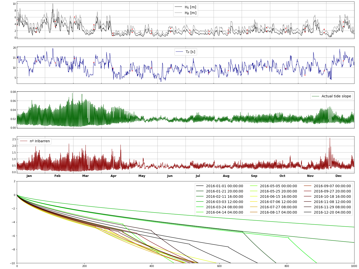
# Select the surfbreak
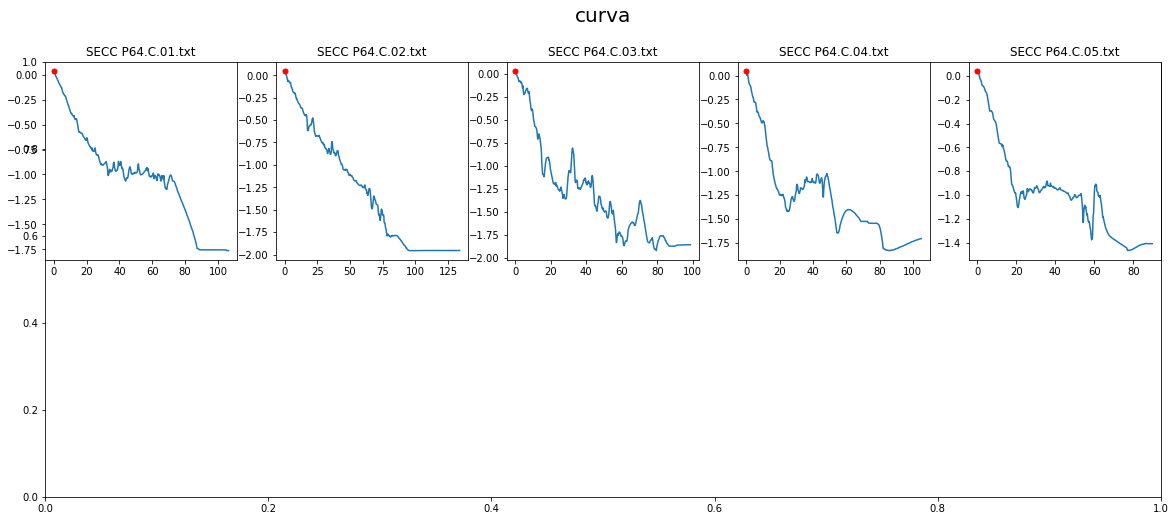
name = 'curva'
surfbreak = surfbreaks_historic.sel(beach=name).to_dataframe()
delta_angle = 340
wf = 0.036
wf_calculated = wf_calc(0.9663, 0.5801)
print('The wf that will be used is: {}'.format(wf))
reconstructed_depth = 8
curva_slope = Slopes(reconstructed_data=surfbreak,
tides=tides,
delta_angle=delta_angle,
wf=wf,
name=name,
reconstructed_depth=reconstructed_depth)
curva_slope.perform_propagation()
curva_slope.moving_profile(year=2016)
curva_slope.data = index(curva_slope.data)
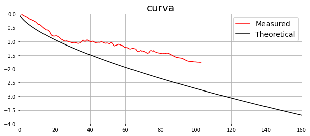
curva_slope.validate_profile(root=op.join(p_data, 'profiles'),
omega=curva_slope.data.groupby('Month').mean().Omega.iloc[7],
diff_sl=1.5)
curva_slope.data['beach'] = name
The values of D50 and wf are, respectively: 0.44761270134600556, 0.048233476184614384
The wf that will be used is: 0.036

 Rolling mean and Ω calculated!!


 Mean wave direction: 5.63806551783085 º


 Mean wind direction: 2.467233362883188 º


 Heights asomerament difference: Hb / Hs : 1.6539946516381308


 Slopes main object constructed!!


 Slopes main object finally constructed!!

<class 'pandas.core.frame.DataFrame'>
DatetimeIndex: 72019 entries, 1979-02-01 02:00:00 to 2020-02-29 20:00:00
Data columns (total 14 columns):
 #   Column      Non-Null Count  Dtype
---  ------      --------------  -----
 0   Hs          72019 non-null  float64
 1   Tp          72019 non-null  float64
 2   Dir         72019 non-null  float64
 3   Spr         72019 non-null  float64
 4   W           72019 non-null  float64
 5   DirW        72019 non-null  float64
 6   DDir        72019 non-null  float64
 7   DDirW       72019 non-null  float64
 8   ocean_tide  72019 non-null  float64
 9   Omega       72019 non-null  float64
 10  H_break     72019 non-null  float64
 11  DDir_R      72019 non-null  float64
 12  Slope       72019 non-null  float64
 13  Iribarren   72019 non-null  float64
dtypes: float64(14)
memory usage: 8.2 MB
None


The values of the profiles plotted are:

                            A         B         C         D     Omega
2016-01-01 00:00:00  0.106525  0.001456  0.266949  0.003002  5.173732
2016-01-21 20:00:00  0.071100  0.000162  0.337801  0.000690  6.945019
2016-02-11 16:00:00  0.070220  0.000153  0.339561  0.000665  6.989020
2016-03-03 12:00:00  0.047452  0.000037  0.385095  0.000259  8.127384
2016-03-24 08:00:00  0.072943  0.000182  0.334113  0.000745  6.852837
2016-04-14 04:00:00  0.093063  0.000632  0.293873  0.001717  5.846836
2016-05-05 00:00:00  0.116427  0.002690  0.247147  0.004528  4.678666
2016-05-25 20:00:00  0.134188  0.008092  0.211623  0.009463  3.790587
2016-06-15 16:00:00  0.139028  0.010924  0.201943  0.011569  3.548583
2016-07-06 12:00:00  0.125598  0.004751  0.228803  0.006626  4.220082
2016-07-27 08:00:00  0.128462  0.005674  0.223076  0.007462  4.076888
2016-08-17 04:00:00  0.133461  0.007736  0.213077  0.009182  3.826926
2016-09-07 00:00:00  0.122524  0.003926  0.234951  0.005832  4.373778
2016-09-27 20:00:00  0.114604  0.002403  0.250793  0.004198  4.769820
2016-10-18 16:00:00  0.120664  0.003499  0.238673  0.005399  4.466822
2016-11-08 12:00:00  0.125399  0.004693  0.229201  0.006571  4.230032
2016-11-29 08:00:00  0.097240  0.000819  0.285520  0.002042  5.637996
2016-12-20 04:00:00  0.117339  0.002847  0.245321  0.004703  4.633029

 0 waves computed...

 20000 waves computed...

 40000 waves computed...

 60000 waves computed...
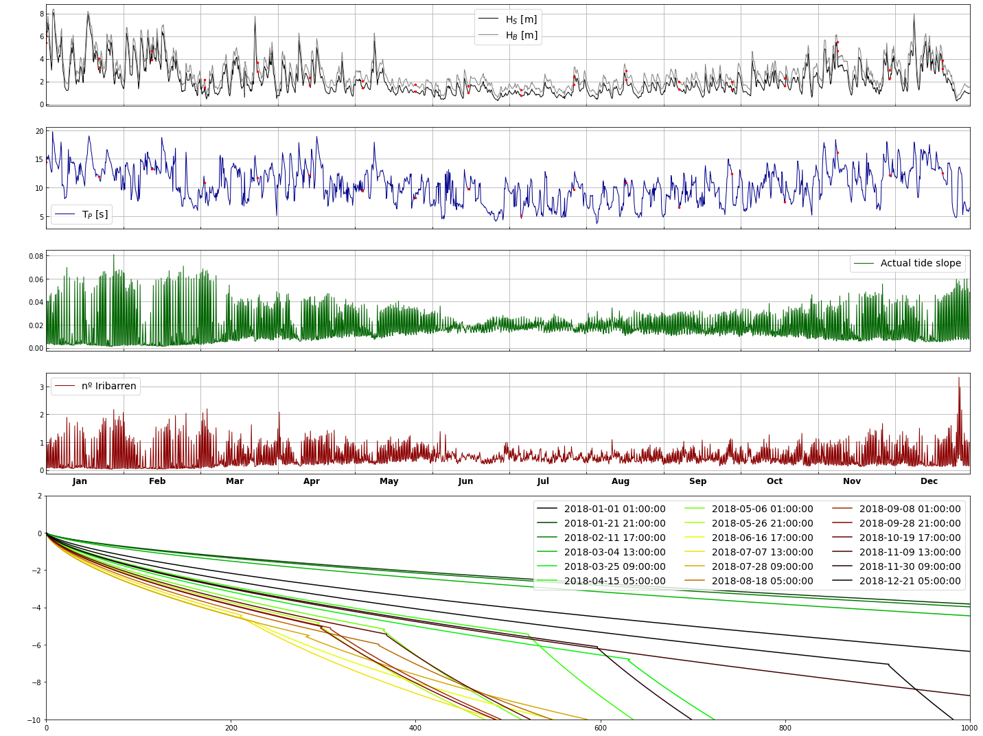
# Select the surfbreak
name = 'brusco'
surfbreak = surfbreaks_historic.sel(beach=name).to_dataframe()
delta_angle = 10
wf = 0.034
wf_calculated = wf_calc(1.2148, 0.5176)
print('The wf that will be used is: {}'.format(wf))
reconstructed_depth = 4
brusco_slope = Slopes(reconstructed_data=surfbreak,
                      tides=tides,
                      delta_angle=delta_angle,
                      wf=wf,
                      name=name,
                      reconstructed_depth=reconstructed_depth)
brusco_slope.perform_propagation()
brusco_slope.moving_profile(year=2018)
brusco_slope.data = index(brusco_slope.data)
brusco_slope.data['beach'] = name
The values of D50 and wf are, respectively: 0.2513298194182252, 0.02556373707462448
The wf that will be used is: 0.034

 Rolling mean and Ω calculated!!


 Mean wave direction: -15.81709037026866 º


 Mean wind direction: -9.365157724579399 º


 Heights asomerament difference: Hb / Hs : 1.4433399236199291


 Slopes main object constructed!!


 Slopes main object finally constructed!!

<class 'pandas.core.frame.DataFrame'>
DatetimeIndex: 72019 entries, 1979-02-01 02:00:00 to 2020-02-29 20:00:00
Data columns (total 14 columns):
 #   Column      Non-Null Count  Dtype
---  ------      --------------  -----
 0   Hs          72019 non-null  float64
 1   Tp          72019 non-null  float64
 2   Dir         72019 non-null  float64
 3   Spr         72019 non-null  float64
 4   W           72019 non-null  float64
 5   DirW        72019 non-null  float64
 6   DDir        72019 non-null  float64
 7   DDirW       72019 non-null  float64
 8   ocean_tide  72019 non-null  float64
 9   Omega       72019 non-null  float64
 10  H_break     72019 non-null  float64
 11  DDir_R      72019 non-null  float64
 12  Slope       72019 non-null  float64
 13  Iribarren   72019 non-null  float64
dtypes: float64(14)
memory usage: 8.2 MB
None


The values of the profiles plotted are:

                            A         B         C         D     Omega
2018-01-01 01:00:00  0.063627  0.000102  0.352746  0.000506  7.318644
2018-01-21 21:00:00  0.038216  0.000021  0.403569  0.000176  8.589214
2018-02-11 17:00:00  0.039716  0.000023  0.400567  0.000188  8.514182
2018-03-04 13:00:00  0.044543  0.000031  0.390915  0.000229  8.272871
2018-03-25 09:00:00  0.092727  0.000619  0.294546  0.001694  5.863638
2018-04-15 05:00:00  0.084101  0.000363  0.311798  0.001184  6.294939
2018-05-06 01:00:00  0.101759  0.001084  0.276482  0.002464  5.412057
2018-05-26 21:00:00  0.110248  0.001834  0.259504  0.003504  4.987605
2018-06-16 17:00:00  0.136723  0.009469  0.206554  0.010513  3.663846
2018-07-07 13:00:00  0.129032  0.005878  0.221937  0.007640  4.048414
2018-07-28 09:00:00  0.138501  0.010573  0.202998  0.011318  3.574942
2018-08-18 05:00:00  0.122457  0.003910  0.235086  0.005816  4.377151
2018-09-08 01:00:00  0.113809  0.002287  0.252381  0.004062  4.809534
2018-09-28 21:00:00  0.114619  0.002405  0.250762  0.004201  4.769058
2018-10-19 17:00:00  0.107080  0.001507  0.265840  0.003072  5.146002
2018-11-09 13:00:00  0.087969  0.000461  0.304062  0.001390  6.101549
2018-11-30 09:00:00  0.086523  0.000421  0.306954  0.001309  6.173860
2018-12-21 05:00:00  0.075109  0.000208  0.329782  0.000815  6.744557

 0 waves computed...

 20000 waves computed...

 40000 waves computed...

 60000 waves computed...
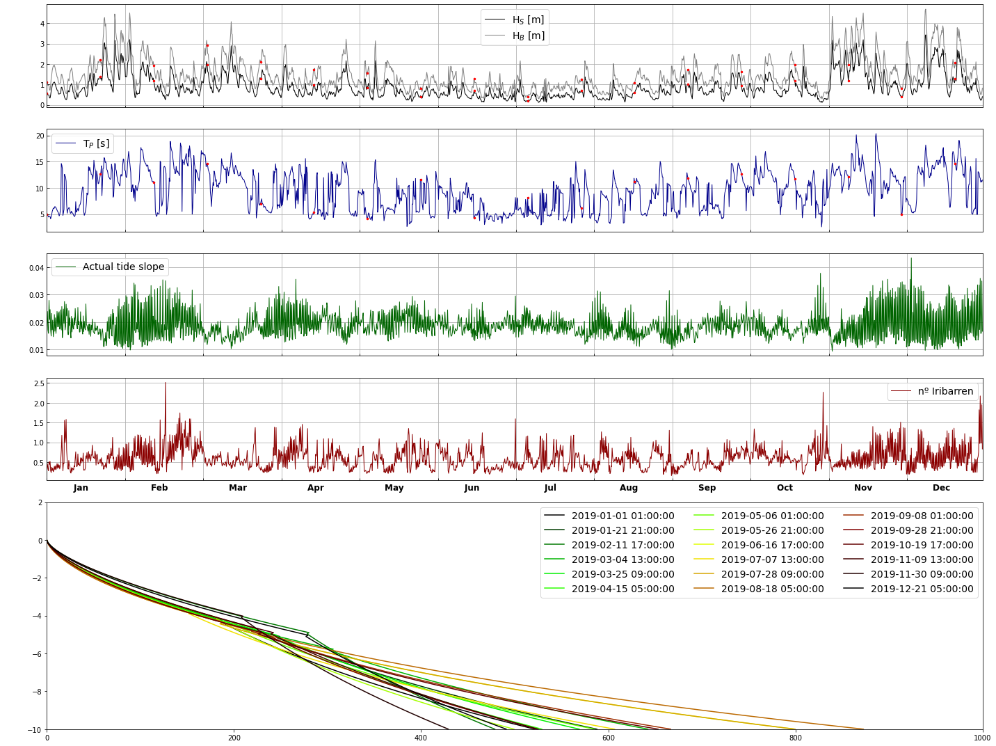
# Select the surfbreak
name = 'laredo'
surfbreak = surfbreaks_historic.sel(beach=name).to_dataframe()
delta_angle = 70
wf = 0.025
print('The wf that will be used is: {}'.format(wf))
reconstructed_depth = 8
laredo_slope = Slopes(reconstructed_data=surfbreak,
                      tides=tides,
                      delta_angle=delta_angle,
                      wf=wf,
                      name=name,
                      reconstructed_depth=reconstructed_depth)
laredo_slope.perform_propagation()
laredo_slope.moving_profile(year=2019)
laredo_slope.data = index(laredo_slope.data)
laredo_slope.data['beach'] = name
The wf that will be used is: 0.025

 Rolling mean and Ω calculated!!


 Mean wave direction: -34.66056423091623 º


 Mean wind direction: -31.01464226066187 º


 Heights asomerament difference: Hb / Hs : 1.8196771203517437


 Slopes main object constructed!!


 Slopes main object finally constructed!!

<class 'pandas.core.frame.DataFrame'>
DatetimeIndex: 72019 entries, 1979-02-01 02:00:00 to 2020-02-29 20:00:00
Data columns (total 14 columns):
 #   Column      Non-Null Count  Dtype
---  ------      --------------  -----
 0   Hs          72019 non-null  float64
 1   Tp          72019 non-null  float64
 2   Dir         72019 non-null  float64
 3   Spr         72019 non-null  float64
 4   W           72019 non-null  float64
 5   DirW        72019 non-null  float64
 6   DDir        72019 non-null  float64
 7   DDirW       72019 non-null  float64
 8   ocean_tide  72019 non-null  float64
 9   Omega       72019 non-null  float64
 10  H_break     72019 non-null  float64
 11  DDir_R      72019 non-null  float64
 12  Slope       72019 non-null  float64
 13  Iribarren   72019 non-null  float64
dtypes: float64(14)
memory usage: 8.2 MB
None


The values of the profiles plotted are:

                            A         B         C         D     Omega
2019-01-01 01:00:00  0.135799  0.008942  0.208401  0.010118  3.710035
2019-01-21 21:00:00  0.140397  0.011891  0.199207  0.012245  3.480172
2019-02-11 17:00:00  0.116678  0.002733  0.246644  0.004576  4.666093
2019-03-04 13:00:00  0.143701  0.014595  0.192598  0.014044  3.314953
2019-03-25 09:00:00  0.138092  0.010308  0.203816  0.011128  3.595408
2019-04-15 05:00:00  0.134205  0.008101  0.211589  0.009470  3.789737
2019-05-06 01:00:00  0.141445  0.012690  0.197111  0.012789  3.427763
2019-05-26 21:00:00  0.132953  0.007496  0.214093  0.008991  3.852328
2019-06-16 17:00:00  0.155161  0.029701  0.169678  0.022597  2.741962
2019-07-07 13:00:00  0.144832  0.015656  0.190335  0.014720  3.258378
2019-07-28 09:00:00  0.155168  0.029714  0.169665  0.022603  2.741620
2019-08-18 05:00:00  0.157863  0.035119  0.164273  0.025279  2.606830
2019-09-08 01:00:00  0.147527  0.018503  0.184945  0.016461  3.123633
2019-09-28 21:00:00  0.133445  0.007728  0.213110  0.009176  3.827753
2019-10-19 17:00:00  0.146626  0.017498  0.186747  0.015857  3.168678
2019-11-09 13:00:00  0.132743  0.007399  0.214513  0.008913  3.862831
2019-11-30 09:00:00  0.115677  0.002568  0.248646  0.004390  4.716141
2019-12-21 05:00:00  0.120995  0.003571  0.238009  0.005474  4.450229

 0 waves computed...

 20000 waves computed...

 40000 waves computed...

 60000 waves computed...
# Select the surfbreak
name = 'forta'
surfbreak = surfbreaks_historic.sel(beach=name).to_dataframe()
delta_angle = 180
wf = 0.015
print('The wf that will be used is: {}'.format(wf))
reconstructed_depth = 6
forta_slope = Slopes(reconstructed_data=surfbreak,
                     tides=tides,
                     delta_angle=delta_angle,
                     wf=wf,
                     name=name,
                     reconstructed_depth=reconstructed_depth)
forta_slope.perform_propagation()
forta_slope.moving_profile(year=2019)
forta_slope.data = index(forta_slope.data)
forta_slope.data['beach'] = name
The wf that will be used is: 0.015

 Rolling mean and Ω calculated!!


 Mean wave direction: -116.51880098209135 º


 Mean wind direction: 9.269694287392666 º


 Heights asomerament difference: Hb / Hs : 1.0


 Slopes main object constructed!!


 Slopes main object finally constructed!!

<class 'pandas.core.frame.DataFrame'>
DatetimeIndex: 72019 entries, 1979-02-01 02:00:00 to 2020-02-29 20:00:00
Data columns (total 14 columns):
 #   Column      Non-Null Count  Dtype
---  ------      --------------  -----
 0   Hs          72019 non-null  float64
 1   Tp          72019 non-null  float64
 2   Dir         72019 non-null  float64
 3   Spr         72019 non-null  float64
 4   W           72019 non-null  float64
 5   DirW        72019 non-null  float64
 6   DDir        72019 non-null  float64
 7   DDirW       72019 non-null  float64
 8   ocean_tide  72019 non-null  float64
 9   Omega       72019 non-null  float64
 10  H_break     72019 non-null  float64
 11  DDir_R      72019 non-null  float64
 12  Slope       72019 non-null  float64
 13  Iribarren   72019 non-null  float64
dtypes: float64(14)
memory usage: 8.2 MB
None


The values of the profiles plotted are:

                            A         B         C         D     Omega
2019-01-01 01:00:00  0.128805  0.005796  0.222390  0.007569  4.059748
2019-01-21 21:00:00  0.134640  0.008322  0.210721  0.009642  3.768020
2019-02-11 17:00:00  0.111211  0.001947  0.257579  0.003647  4.939470
2019-03-04 13:00:00  0.136840  0.009538  0.206320  0.010564  3.658000
2019-03-25 09:00:00  0.132296  0.007196  0.215409  0.008749  3.885223
2019-04-15 05:00:00  0.127901  0.005480  0.224198  0.007290  4.104940
2019-05-06 01:00:00  0.134644  0.008324  0.210712  0.009644  3.767808
2019-05-26 21:00:00  0.128048  0.005530  0.223904  0.007335  4.097592
2019-06-16 17:00:00  0.155580  0.030483  0.168840  0.022993  2.721004
2019-07-07 13:00:00  0.144004  0.014872  0.191991  0.014222  3.299780
2019-07-28 09:00:00  0.154929  0.029277  0.170143  0.022380  2.753572
2019-08-18 05:00:00  0.156040  0.031365  0.167920  0.023436  2.698010
2019-09-08 01:00:00  0.143375  0.014303  0.193251  0.013855  3.331266
2019-09-28 21:00:00  0.127429  0.005322  0.225143  0.007149  4.128573
2019-10-19 17:00:00  0.142970  0.013948  0.194060  0.013625  3.351503
2019-11-09 13:00:00  0.130809  0.006562  0.218383  0.008225  3.959571
2019-11-30 09:00:00  0.111088  0.001932  0.257824  0.003628  4.945598
2019-12-21 05:00:00  0.113364  0.002225  0.253272  0.003988  4.831794

 0 waves computed...

 20000 waves computed...

 40000 waves computed...

 60000 waves computed...
data = pd.concat([farolillo_slope.data, bederna_slope.data, oyambre_slope.data,
                  locos_slope.data, canallave_slope.data, valdearenas_slope.data, madero_slope.data,
                  segunda_slope.data, primera_slope.data,
                  pueblo_slope.data, curva_slope.data,
                  brusco_slope.data, laredo_slope.data, forta_slope.data])
data.info()
<class 'pandas.core.frame.DataFrame'>
DatetimeIndex: 1008266 entries, 1979-02-01 02:00:00 to 2020-02-29 20:00:00
Data columns (total 27 columns):
 #   Column           Non-Null Count    Dtype
---  ------           --------------    -----
 0   Hs               1008266 non-null  float64
 1   Tp               1008266 non-null  float64
 2   Dir              1008266 non-null  float64
 3   Spr              1008266 non-null  float64
 4   W                1008266 non-null  float64
 5   DirW             1008266 non-null  float64
 6   DDir             1008266 non-null  float64
 7   DDirW            1008266 non-null  float64
 8   ocean_tide       1008266 non-null  float64
 9   Omega            1008266 non-null  float64
 10  H_break          1008266 non-null  float64
 11  DDir_R           1008266 non-null  float64
 12  Slope            1008091 non-null  float64
 13  Iribarren        1008091 non-null  float64
 14  Hb_index         1008266 non-null  float64
 15  Tp_index         1008266 non-null  float64
 16  Spr_index        1008266 non-null  float64
 17  Iribarren_index  1008266 non-null  float64
 18  Dir_index        1008266 non-null  float64
 19  DirW_index       1008266 non-null  float64
 20  Index            1008266 non-null  float64
 21  Hour             1008266 non-null  int64
 22  Day_Moment       1008266 non-null  object
 23  Month            1008266 non-null  int64
 24  Season           1008266 non-null  object
 25  Year             1008266 non-null  int64
 26  beach            1008266 non-null  object
dtypes: float64(21), int64(3), object(3)
memory usage: 215.4+ MB
data.to_pickle(op.join(p_data, 'reconstructed', 'surfbreaks_reconstructed_final.pkl'))