1. Maximum Dissimilarity Algorithm (MDA)
Once the wave reanalysis data has been calibrated and validated (refer to the repository CalValWaves for more detailed information in this way), a hybrid downscaling method to shallower water is proposed so a high resolution wave climate in the coast can be obtained all over the world. This resolution depends on two main factors:
The resolution of the bathymetry used, which depends on the data available, as a global bathymetry grid is proportioned by GEBCO and will be used here so it can be extended worldwide, but more detailed grids can be obtained (also shown in this project).
The computational capacity of the machines used (it will make sense in the propagation step).
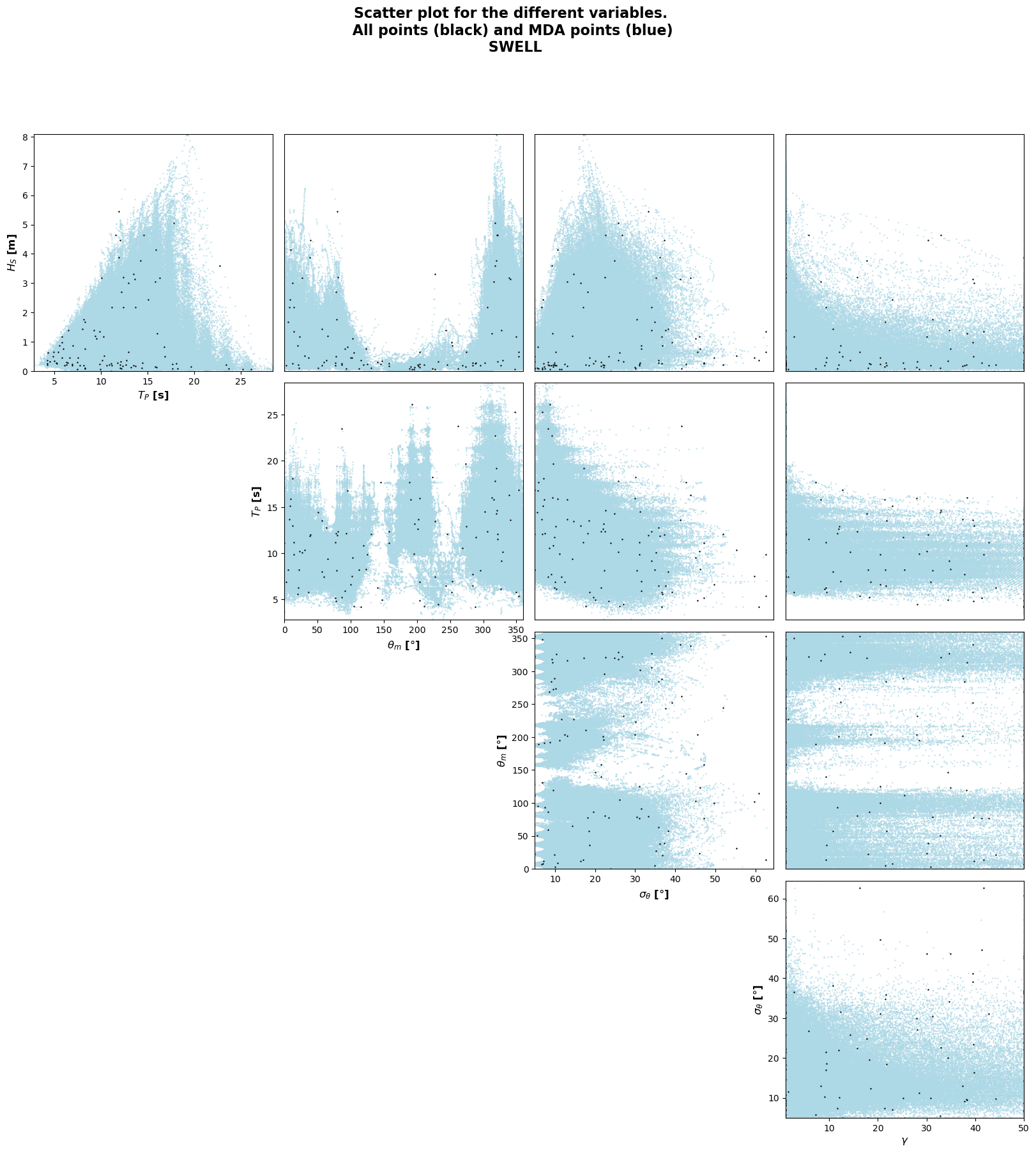
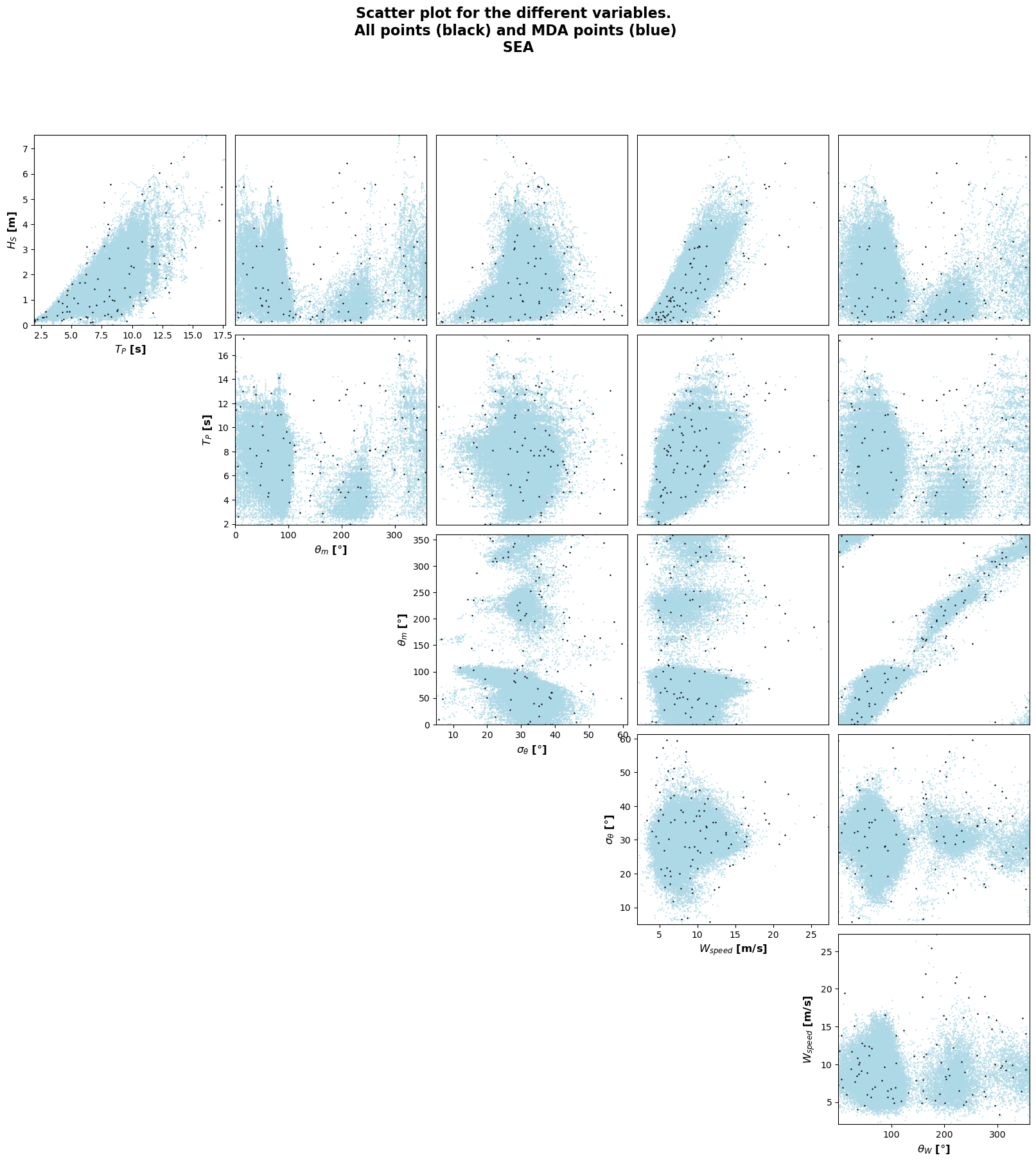
In this way, the first step to carry out this downscaling method is the selection of the maximum dissimilar cases, so the posterior propagation of the cases can be performed correctly (Javier Tausia, 2020, main directory of the repository). For this purpose, a certain number of windseas and swells is selected from the total set of 40 years so these two type of waves can be more or less represented. The way this selection is performed is described in the image below and in the previously cited work:
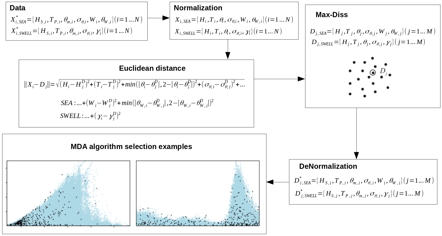
This sketch shows the workflow followed in the selection step. The data is firstly normalized for the correct performance of the algorithm, then the euclidean distance is used for the calculation of the distance between the different vectors in the dataset. Finally, the selected data is de-normalized so it can be used and plotted together with the original information.
As it can be seen, the variables used in the definition of the windseas and the swells are different, and it is due to the fact that windseas and swells do not propagate equally and their characteristics are not the same. The variables used are:
where \(H_S\) is the significant wave height, \(T_P\) is the peak period, \(\theta_m\) is the mean wave direction, \(\sigma_\theta\) is the dispersion or cleanliness, \(W\) is the wind magnitude, \(\theta_W\) is the wind direction and \(\gamma\) (jonswap) gives an idea about the shape of the wave spectra.
# import the modules
import sys
import os
import os.path as op
import pandas as pd
import numpy as np
import matplotlib.pyplot as plt
from mda_functions import MaxDiss_Simplified_NoThreshold as MDA
The first thing that is done is the selection of the number of cases that will be selected, worth the redundancy:
num_centroids = 100
Notice that the algorithm will not take too much time even if the number of cases is too large, maybe a few minutes, but when doing the propagations, the computational effort is larger, so be careful. Next, files are loaded and the preprocessing is performed:
p_hind = op.join(os.getcwd(), '..', 'data', 'hindcast')
dataframe_total = pd.read_pickle(op.join(p_hind, 'csiro_dataframe_oahu_sat_corr.pkl'))
# this sat_corr dataframe is the one obtained in CalValWaves, exactly the same!!
# two copies are done for the selection of the seas and the swells
sea = dataframe_total.copy()
swell = dataframe_total.copy()
print(dataframe_total.info())
<class 'pandas.core.frame.DataFrame'>
DatetimeIndex: 362304 entries, 1980-01-01 00:00:00 to 2021-04-30 23:00:00
Data columns (total 29 columns):
 #   Column     Non-Null Count   Dtype
---  ------     --------------   -----
 0   Hs         362304 non-null  float64
 1   Tm_01      292920 non-null  float32
 2   Tm_02      362304 non-null  float32
 3   Tp         362304 non-null  float32
 4   DirM       362304 non-null  float32
 5   DirP       362304 non-null  float32
 6   Spr        362304 non-null  float32
 7   Nwp        362304 non-null  float32
 8   U10        362304 non-null  float32
 9   V10        362304 non-null  float32
 10  W          362304 non-null  float64
 11  DirW       362298 non-null  float64
 12  Hsea       362304 non-null  float64
 13  Hswell1    362304 non-null  float64
 14  Hswell2    362304 non-null  float64
 15  Hswell3    362304 non-null  float64
 16  Tpsea      244833 non-null  float32
 17  Tpswell1   361904 non-null  float32
 18  Tpswell2   345998 non-null  float32
 19  Tpswell3   297651 non-null  float32
 20  Dirsea     244833 non-null  float32
 21  Dirswell1  361904 non-null  float32
 22  Dirswell2  345998 non-null  float32
 23  Dirswell3  297651 non-null  float32
 24  Sprsea     244833 non-null  float32
 25  Sprswell1  361904 non-null  float32
 26  Sprswell2  345998 non-null  float32
 27  Sprswell3  297651 non-null  float32
 28  Hs_cal     362304 non-null  float64
dtypes: float32(21), float64(8)
memory usage: 53.9 MB
None
For the preprocessing step, two different sets of data must be used:
For the seas, a dataframe with the required variables is obtained.
For the swells, all the different partitions must be joined (3 in this case), and all the variables must be included in this set.
Here, the code might not be touched except the case that more swells exist in the wave reanalysis that wanna be added in the selection of the swells dataset.
# SEA DATAFRAME
xys_sea = ['Hsea', 'Tpsea', 'Dirsea', 'Sprsea', 'W', 'DirW']
sea = sea[xys_sea].dropna(axis=0, how='any')
# limited dispersion threshold so the analysis is coherent
sea['Sprsea'][sea['Sprsea']<5] = 5
# SWELL DATAFRAME
xys_swell = ['Tm_02',
             'Hswell1', 'Tpswell1', 'Dirswell1', 'Sprswell1',
             'Hswell2', 'Tpswell2', 'Dirswell2', 'Sprswell2',
             'Hswell3', 'Tpswell3', 'Dirswell3', 'Sprswell3']
swell = swell[xys_swell]
swell = pd.DataFrame({'Tm_02': np.repeat(swell['Tm_02'], 3),
                      'Hswell': np.concatenate((swell['Hswell1'].values,
                                                swell['Hswell2'].values,
                                                swell['Hswell3'].values),
                                               axis=0),
                      'Tpswell': np.concatenate((swell['Tpswell1'].values,
                                                 swell['Tpswell2'].values,
                                                 swell['Tpswell3'].values),
                                                axis=0),
                      'Dirswell': np.concatenate((swell['Dirswell1'].values,
                                                  swell['Dirswell2'].values,
                                                  swell['Dirswell3'].values),
                                                 axis=0),
                      'Sprswell': np.concatenate((swell['Sprswell1'].values,
                                                  swell['Sprswell2'].values,
                                                  swell['Sprswell3'].values),
                                                 axis=0)})
swell = swell.dropna(axis=0, how='any')
# limited dispersion threshold so the analysis is coherent
swell['Sprswell'][swell['Sprswell']<5] = 5
swell['Gamma'] = np.power(swell['Tpswell'].values/\
                          (swell['Tm_02'].values * 1.411),
                          -12.5439)
# limited shape of the spectrum threshold so the analysis is coherent
swell['Gamma'][swell['Gamma']<1] = 1
swell['Gamma'][swell['Gamma']>50] = 50
<ipython-input-7-5884f8f5e07d>:31: SettingWithCopyWarning:
A value is trying to be set on a copy of a slice from a DataFrame

See the caveats in the documentation: https://pandas.pydata.org/pandas-docs/stable/user_guide/indexing.html#returning-a-view-versus-a-copy
  swell['Gamma'][swell['Gamma']<1] = 1
<ipython-input-7-5884f8f5e07d>:32: SettingWithCopyWarning:
A value is trying to be set on a copy of a slice from a DataFrame

See the caveats in the documentation: https://pandas.pydata.org/pandas-docs/stable/user_guide/indexing.html#returning-a-view-versus-a-copy
  swell['Gamma'][swell['Gamma']>50] = 50
data = [sea, swell]
labels = [['Hsea', 'Tpsea', 'Dirsea', 'Sprsea', 'W', 'DirW'],
          ['Hswell', 'Tpswell', 'Dirswell', 'Sprswell', 'Gamma']]
names = [['$H_S$ [m]', '$T_P$ [s]', '$\u03B8_{m}$ [$\degree$]',
          '$\sigma_{\u03B8}$ [$\degree$]', '$W_{speed}$ [m/s]', '$\u03B8_{W}$ [$\degree$]'],
         ['$H_S$ [m]', '$T_P$ [s]', '$\u03B8_{m}$ [$\degree$]',
          '$\sigma_{\u03B8}$ [$\degree$]', '$\gamma$']]
title = ['sea', 'swell']
# input values for the MDA algorithm functions in functions.py
scalars = [[0,1,3,4], [0,1,3,4]]
directionals = [[2,5], [2]]
for wave in range(0,2):

    dataframe = data[wave]
    xys = labels[wave]
    xys_names = names[wave]
    scalar = scalars[wave]
    directional = directionals[wave]

    dataframe = dataframe[xys]
    dataarray = dataframe.to_numpy()

    # SUBSET
    subarray = MDA(dataarray, num_centroids, scalar, directional)
    subset = pd.DataFrame(subarray, columns=xys)

    # Scatter plot MDA centroids
    fig, axs = plt.subplots(len(xys)-1, len(xys)-1, figsize = (20,20))
    plt.subplots_adjust(wspace=0.05, hspace=0.05)
    plt.suptitle('Scatter plot for the different variables. \n ' +
                 'All points (black) and MDA points (blue) \n ' +
                 title[wave].upper(), fontsize=16, fontweight='bold')

    for i, item in enumerate(xys):
        xys_copy = xys.copy()
        xys_names_copy = xys_names.copy()
        for p in range(i+1):
            xys_copy.pop(0)
            xys_names_copy.pop(0)
        for j, jtem in enumerate(xys_copy):
            axs[i,j+i].scatter(dataframe[jtem], dataframe[item], marker=".",
                               s=1, color = 'lightblue')
            axs[i,j+i].scatter(subset[jtem], subset[item], marker=".",
                               s=2,  color = 'k')
            axs[i,j+i].set_xlim(min(dataframe[jtem]), max(dataframe[jtem]))
            axs[i,j+i].set_ylim(min(dataframe[item]), max(dataframe[item]))
            if i==j+i:
                axs[i,j+i].set_xlabel(xys_names_copy[j], fontsize=12,
                                      fontweight='bold')
                axs[i,j+i].set_ylabel(xys_names[i], fontsize=12,
                                      fontweight='bold')
            else:
                axs[i,j+i].set_xticks([])
                axs[i,j+i].set_yticks([])
            len_xys = len(xys)-len(xys_copy)-1
            if len_xys != 0:
                for k in range(len_xys):
                    axs[i,k].axis('off')
    # show results
    plt.show()

    # data is saved in the data/hindcast folder
    subset.to_pickle(op.join(p_hind, title[wave] + '_cases_' + str(num_centroids) + '_oahu.pkl'))
MaxDiss waves parameters: 244833 --> 100

   MDA centroids: 050/100

Number of centroids computed: 50


   MDA centroids: 100/100

Number of centroids computed: 100
MaxDiss waves parameters: 1005553 --> 100

   MDA centroids: 050/100

Number of centroids computed: 50


   MDA centroids: 100/100

Number of centroids computed: 100