5. Slopes analysis, SOM…
# common
import sys
import os
import os.path as op

# basic
import xarray as xr
import numpy as np
import pandas as pd
from datetime import timedelta as td
from matplotlib import pyplot as plt
from pandas.plotting import register_matplotlib_converters

# interactive
from ipywidgets import interactive

# advanced
import plotly.express as px
import plotly.graph_objects as go
import plotly.figure_factory as ff
import dash  # (version 1.12.0) pip install dash
import dash_core_components as dcc
import dash_html_components as html
from dash.dependencies import Input, Output

# warnings
import warnings
warnings.filterwarnings("ignore")

# dev library
sys.path.insert(0, os.getcwd())

# RBF module
from slopes import Slopes_SOM
from slopes import consult
# pip renders for jupyter book
import plotly.io as pio
pio.renderers.default = "notebook"
# load the data
data = pd.read_pickle(op.join(os.getcwd(), '..', 'data', 'reconstructed',
                              'surfbreaks_reconstructed_final.pkl'))
data['Index'] = data['Index'].where(data['Index']<1, 1) * 10
data = data.dropna(how='any', axis=0)

data.info()
<class 'pandas.core.frame.DataFrame'>
DatetimeIndex: 1008091 entries, 1979-02-01 02:00:00 to 2020-02-29 20:00:00
Data columns (total 27 columns):
 #   Column           Non-Null Count    Dtype
---  ------           --------------    -----
 0   Hs               1008091 non-null  float64
 1   Tp               1008091 non-null  float64
 2   Dir              1008091 non-null  float64
 3   Spr              1008091 non-null  float64
 4   W                1008091 non-null  float64
 5   DirW             1008091 non-null  float64
 6   DDir             1008091 non-null  float64
 7   DDirW            1008091 non-null  float64
 8   ocean_tide       1008091 non-null  float64
 9   Omega            1008091 non-null  float64
 10  H_break          1008091 non-null  float64
 11  DDir_R           1008091 non-null  float64
 12  Slope            1008091 non-null  float64
 13  Iribarren        1008091 non-null  float64
 14  Hb_index         1008091 non-null  float64
 15  Tp_index         1008091 non-null  float64
 16  Spr_index        1008091 non-null  float64
 17  Iribarren_index  1008091 non-null  float64
 18  Dir_index        1008091 non-null  float64
 19  DirW_index       1008091 non-null  float64
 20  Index            1008091 non-null  float64
 21  Hour             1008091 non-null  int64
 22  Day_Moment       1008091 non-null  object
 23  Month            1008091 non-null  int64
 24  Season           1008091 non-null  object
 25  Year             1008091 non-null  int64
 26  beach            1008091 non-null  object
dtypes: float64(21), int64(3), object(3)
memory usage: 215.4+ MB
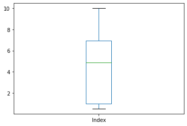
data.Index.plot.box()
<AxesSubplot:>
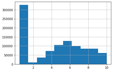
data.Hb_index.hist()
<AxesSubplot:>
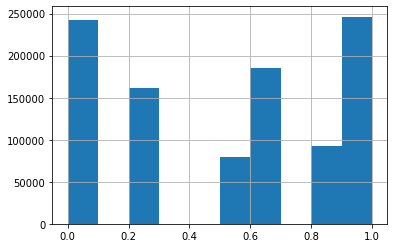
data.Index.hist()
<AxesSubplot:>
consult(data=data,
        beaches=['segunda', 'laredo', 'forta'],
        day='2017-01-13',
        columns=['H_break', 'Hb_index', 'Index'])
| H_break | Hb_index | Index | beach | |
|---|---|---|---|---|
| 2017-01-13 03:00:00 | 3.857180 | 0.3 | 3.376 | segunda |
| 2017-01-13 08:00:00 | 3.926694 | 0.3 | 2.532 | segunda |
| 2017-01-13 13:00:00 | 3.804837 | 0.3 | 3.376 | segunda |
| 2017-01-13 18:00:00 | 4.560021 | 0.0 | 1.000 | segunda |
| 2017-01-13 23:00:00 | 3.389903 | 0.5 | 5.088 | segunda |
| 2017-01-13 03:00:00 | 3.747338 | 0.3 | 2.664 | laredo |
| 2017-01-13 08:00:00 | 3.819149 | 0.3 | 2.664 | laredo |
| 2017-01-13 13:00:00 | 3.717768 | 0.5 | 4.384 | laredo |
| 2017-01-13 18:00:00 | 4.273107 | 0.3 | 3.776 | laredo |
| 2017-01-13 23:00:00 | 3.435028 | 0.5 | 4.608 | laredo |
| 2017-01-13 03:00:00 | 1.646689 | 0.7 | 4.128 | forta |
| 2017-01-13 08:00:00 | 1.679265 | 0.7 | 5.216 | forta |
| 2017-01-13 13:00:00 | 1.637391 | 0.7 | 7.568 | forta |
| 2017-01-13 18:00:00 | 2.068835 | 1.0 | 9.438 | forta |
| 2017-01-13 23:00:00 | 1.480459 | 0.7 | 8.250 | forta |
consult(data=data,
        beaches=['segunda', 'laredo', 'forta'],
        day='2019-12-22',
        columns=['H_break', 'Hb_index', 'Index'])
| H_break | Hb_index | Index | beach | |
|---|---|---|---|---|
| 2019-12-22 01:00:00 | 3.646619 | 0.5 | 4.320 | segunda |
| 2019-12-22 06:00:00 | 3.164886 | 0.5 | 4.860 | segunda |
| 2019-12-22 11:00:00 | 2.948261 | 0.8 | 6.264 | segunda |
| 2019-12-22 16:00:00 | 3.183460 | 0.5 | 4.320 | segunda |
| 2019-12-22 21:00:00 | 2.933703 | 0.8 | 5.856 | segunda |
| 2019-12-22 01:00:00 | 3.782744 | 0.3 | 3.664 | laredo |
| 2019-12-22 06:00:00 | 3.431986 | 0.5 | 5.382 | laredo |
| 2019-12-22 11:00:00 | 3.289403 | 0.5 | 5.058 | laredo |
| 2019-12-22 16:00:00 | 3.717900 | 0.5 | 4.496 | laredo |
| 2019-12-22 21:00:00 | 3.537950 | 0.5 | 4.976 | laredo |
| 2019-12-22 01:00:00 | 1.630818 | 0.7 | 4.212 | forta |
| 2019-12-22 06:00:00 | 1.441102 | 0.7 | 4.356 | forta |
| 2019-12-22 11:00:00 | 1.392555 | 0.7 | 4.212 | forta |
| 2019-12-22 16:00:00 | 1.624850 | 0.7 | 4.212 | forta |
| 2019-12-22 21:00:00 | 1.505351 | 0.7 | 4.356 | forta |
consult(data=data,
        beaches=['brusco', 'canallave', 'laredo'],
        day='2003-06-20',
        columns=['H_break', 'Hb_index', 'Index'])
| H_break | Hb_index | Index | beach | |
|---|---|---|---|---|
| 2003-06-20 02:00:00 | 2.131825 | 1.0 | 6.798 | canallave |
| 2003-06-20 07:00:00 | 1.979701 | 1.0 | 5.168 | canallave |
| 2003-06-20 12:00:00 | 2.064915 | 1.0 | 5.168 | canallave |
| 2003-06-20 17:00:00 | 2.103380 | 1.0 | 1.000 | canallave |
| 2003-06-20 22:00:00 | 1.854655 | 1.0 | 7.106 | canallave |
| 2003-06-20 02:00:00 | 1.792632 | 1.0 | 6.886 | brusco |
| 2003-06-20 07:00:00 | 1.678462 | 0.7 | 3.472 | brusco |
| 2003-06-20 12:00:00 | 1.858943 | 1.0 | 1.000 | brusco |
| 2003-06-20 17:00:00 | 1.997746 | 1.0 | 1.000 | brusco |
| 2003-06-20 22:00:00 | 1.703752 | 1.0 | 1.000 | brusco |
| 2003-06-20 02:00:00 | 1.234815 | 0.7 | 1.000 | laredo |
| 2003-06-20 07:00:00 | 1.291503 | 0.7 | 1.000 | laredo |
| 2003-06-20 12:00:00 | 1.678732 | 0.7 | 1.000 | laredo |
| 2003-06-20 17:00:00 | 1.842311 | 1.0 | 1.000 | laredo |
| 2003-06-20 22:00:00 | 1.498014 | 0.7 | 1.000 | laredo |
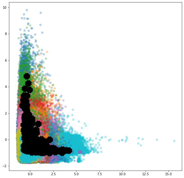
def plot_scatter(x, y):
    fig = px.scatter(data[::100], x=x, y=y, color='beach')
    fig.show()

interactive_plot = interactive(plot_scatter,
                               x=data.columns,
                               y=data.columns)
interactive_plot
def plot_bar(grouper, variable):
    fig = px.bar(data.groupby([grouper, 'beach']).mean().reset_index(),
                 y=variable,
                 x=grouper,
                 color='beach',
                 barmode='group')
    fig.show()

interactive_plot = interactive(plot_bar,
                               grouper=['Hour', 'Day_Moment', 'Month', 'Season', 'Year'],
                               variable=data.columns)
interactive_plot
def plot_box(period, y):
    data_box = data.copy()
    if isinstance(period, np.int64):
        fig = px.box(data_box.where(data_box['Month']==period).dropna(how='all', axis=0),
                     x='beach', y=y, title='Month: '+str(period))
    elif period=='all':
        fig = px.box(data_box, x='beach', y=y, title='Points: '+period)
    elif period in ['Winter', 'Spring', 'Summer', 'Autumn']:
        fig = px.box(data_box.where(data_box['Season']==period).dropna(how='all', axis=0),
                     x='beach', y=y, title='Season: '+period)
    else:
        fig = px.box(data_box.where(data_box['Day_Moment']==period).dropna(how='all', axis=0),
                     x='beach', y=y, title='Day moment: '+period)
    fig.show()

period = ['all'] + list(data.Season.unique()) + list(data.Month.unique()) + list(data.Day_Moment.unique())

interactive_plot = interactive(plot_box,
                               period=period,
                               y=data.columns)
interactive_plot
def plot_hist(period, x):
    data_hist = data[::100].copy()
    if isinstance(period, np.int64):
        fig = px.histogram(data_hist.where(data_hist['Month']==period).dropna(how='all', axis=0),
                           x=x, color='beach', marginal='box',
                           hover_data=data.columns, title='Month: '+str(period))
    elif period=='all':
        fig = px.histogram(data_hist,
                           x=x, color='beach', marginal='box',
                           hover_data=data.columns, title='Points: '+period)
    elif period in ['Winter', 'Spring', 'Summer', 'Autumn']:
        fig = px.histogram(data_hist.where(data_hist['Season']==period).dropna(how='all', axis=0),
                           x=x, color='beach', marginal='box',
                           hover_data=data.columns, title='Season: '+period)
    else:
        fig = px.histogram(data_hist.where(data_hist['Day_Moment']==period).dropna(how='all', axis=0),
                           x=x, color='beach', marginal='box',
                           hover_data=data.columns, title='Day moment: '+period)
    fig.show()

period = ['all'] + list(data.Season.unique()) + list(data.Month.unique()) + list(data.Day_Moment.unique())

interactive_plot = interactive(plot_hist,
                               period=period,
                               x=data.columns)
interactive_plot
def plot_prob(beach):
    histcolor = ['blue', 'green', 'yellow', 'orange', 'red', 'purple', 'black']
    data_prob = data.where(data['beach']==beach).dropna(how='all', axis=0).copy()
    data_prob = data_prob.groupby([data_prob.index.dayofyear,
                                   pd.cut(data_prob['Index'],
                                          [0,1,3,5,7,8,9,10],
                                          right=True)])\
                .count().mean(axis=1) / (len(data_prob)/366)
    data_prob.name = 'Probability of RSI'
    fig = px.histogram(data_prob.reset_index(),
                       x='level_0', y='Probability of RSI',
                       color='Index',
                       color_discrete_map={key: value for (key, value) in zip(
                           data_prob.reset_index()['Index'].unique(),
                           histcolor)},
                       nbins=366, range_y=[0,1],
                       labels={'level_0': 'Day of year'},
                       title='Beach: ' + beach, width=900, height=400)
    fig.show()

interactive_plot = interactive(plot_prob,
                               beach=data.beach.unique())
interactive_plot
def plot_prob(beach, ini_year, end_year):
    histcolor = ['blue', 'green', 'yellow', 'orange', 'red', 'purple', 'black']
    data_prob = data.where(data['beach']==beach).dropna(how='all', axis=0).copy()
    data_prob = data.where((data['Year']>=ini_year) & (data['Year']<=end_year))\
                .dropna(how='all', axis=0).copy()
    data_prob = data_prob.groupby([pd.Grouper(freq='M'),
                                   pd.cut(data_prob['Index'],
                                          [0,1,3,5,7,8,9,10],
                                          right=True)])\
                .count().mean(axis=1) / (len(data_prob)/(12*(end_year-ini_year + 1)))
    data_prob.name = 'Probability of RSI'
    fig = px.histogram(data_prob.reset_index(),
                       x='level_0', y='Probability of RSI',
                       color='Index',
                       color_discrete_map={key: value for (key, value) in zip(
                           data_prob.reset_index()['Index'].unique(),
                           histcolor)},
                       nbins=12*int(end_year-ini_year + 1), range_y=[0,1],
                       labels={'level_0': 'Historical month'},
                       title='Beach: ' + beach, width=900, height=400)
    fig.show()

interactive_plot = interactive(plot_prob,
                               beach=data.beach.unique(),
                               ini_year=data.Year.unique(),
                               end_year=data.Year.unique())
interactive_plot
def plot_prob_grouper(beach, grouper):
    histcolor = ['blue', 'green', 'yellow', 'orange', 'red', 'purple', 'black']
    data_prob = data.where(data['beach']==beach).dropna(how='all', axis=0).copy()
    data_prob = data_prob.groupby([data_prob[grouper],
                                   pd.cut(data_prob['Index'],
                                          [0,1,3,5,7,8,9,10],
                                          right=True)])\
                .count().mean(axis=1) / (len(data_prob)/len(data[grouper].unique()))
    data_prob.name = 'Probability of RSI'
    fig = px.histogram(data_prob.reset_index(),
                       x=grouper, y='Probability of RSI',
                       color='Index',
                       color_discrete_map={key: value for (key, value) in zip(
                           data_prob.reset_index()['Index'].unique(),
                           histcolor)},
                       range_y=[0,1], nbins=len(data[grouper].unique()),
                       labels={'level_0': grouper},
                       title='Beach: ' + beach, width=900, height=400)
    fig.show()

grouper = ['Month', 'Season', 'Year']

interactive_plot = interactive(plot_prob_grouper,
                               beach=data.beach.unique(),
                               grouper=grouper)
interactive_plot
def plot_rose(beach):
    data_prob = data.where(data['beach']==beach).dropna(how='all', axis=0).copy()
    data_prob = data_prob.groupby([pd.cut(data_prob['Dir'],
                                          [0,20,40,60,80,100,120,140,160,180,
                                           200,220,240,260,280,300,320,340,360],
                                          right=True),
                                   pd.cut(data_prob['Tp'],
                                          [0,6,8,10,12,14,16,18,24],
                                          right=True)]).mean()
    data_prob = data_prob['H_break'].rename('H_break_value', inplace=True).reset_index()
    data_prob = data_prob.astype({'Dir': 'str', 'Tp': 'str'}, copy=True)
    fig = px.bar_polar(data_prob, r='H_break_value', theta='Dir',
                       color='Tp', color_discrete_sequence=px.colors.sequential.Plasma_r)
    fig.show()

interactive_plot = interactive(plot_rose,
                               beach=data.beach.unique())
interactive_plot
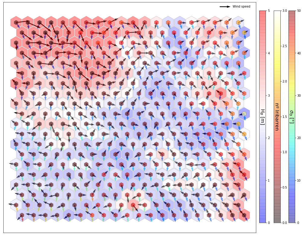
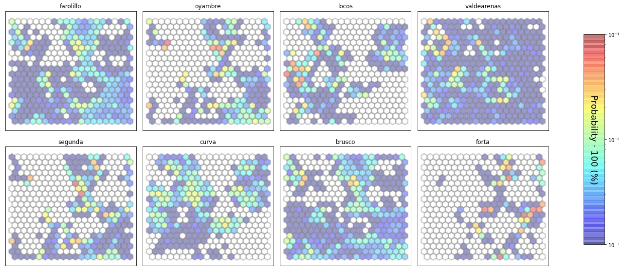
slopes_som = Slopes_SOM(data)
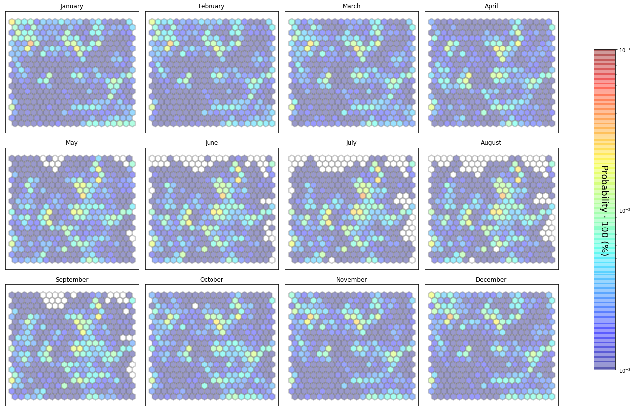
som, data_mean, data_count = slopes_som.train(som_shape=(20,20), sigma=0.8, learning_rate=0.5,
num_iteration=80000, plot_results=True)
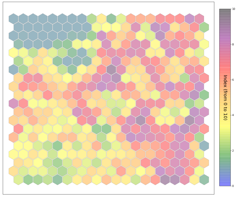
slopes_som.plot_results(som, data_mean, data_count, plot_beaches=True, plot_months=True)
The following data will be trained:


<class 'pandas.core.frame.DataFrame'>
DatetimeIndex: 1008091 entries, 1979-02-01 02:00:00 to 2020-02-29 20:00:00
Data columns (total 27 columns):
 #   Column           Non-Null Count    Dtype
---  ------           --------------    -----
 0   Hs               1008091 non-null  float64
 1   Tp               1008091 non-null  float64
 2   Dir              1008091 non-null  float64
 3   Spr              1008091 non-null  float64
 4   W                1008091 non-null  float64
 5   DirW             1008091 non-null  float64
 6   DDir             1008091 non-null  float64
 7   DDirW            1008091 non-null  float64
 8   ocean_tide       1008091 non-null  float64
 9   Omega            1008091 non-null  float64
 10  H_break          1008091 non-null  float64
 11  DDir_R           1008091 non-null  float64
 12  Slope            1008091 non-null  float64
 13  Iribarren        1008091 non-null  float64
 14  Hb_index         1008091 non-null  float64
 15  Tp_index         1008091 non-null  float64
 16  Spr_index        1008091 non-null  float64
 17  Iribarren_index  1008091 non-null  float64
 18  Dir_index        1008091 non-null  float64
 19  DirW_index       1008091 non-null  float64
 20  Index            1008091 non-null  float64
 21  Hour             1008091 non-null  int64
 22  Day_Moment       1008091 non-null  object
 23  Month            1008091 non-null  int64
 24  Season           1008091 non-null  object
 25  Year             1008091 non-null  int64
 26  beach            1008091 non-null  object
dtypes: float64(21), int64(3), object(3)
memory usage: 215.4+ MB
None
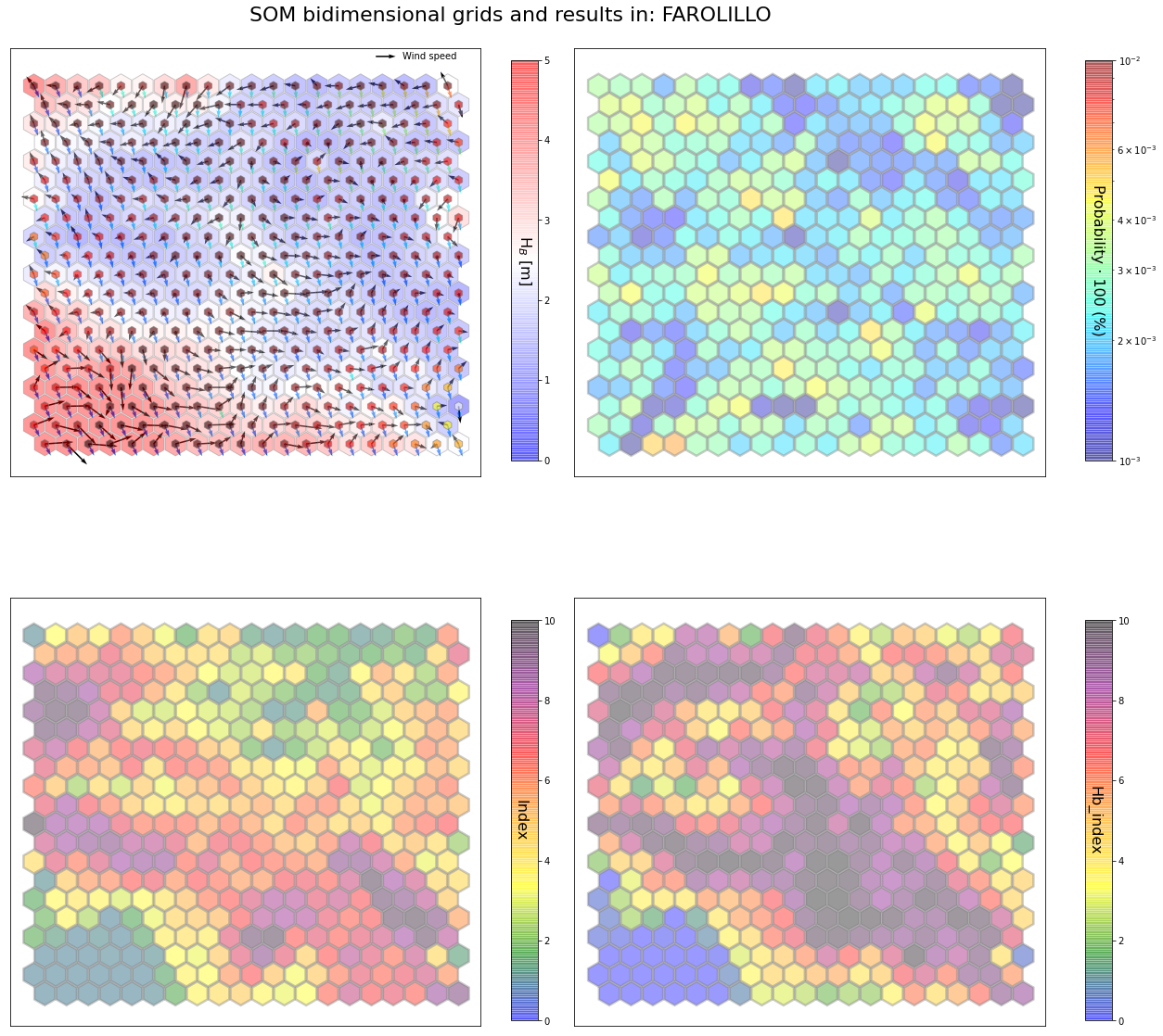
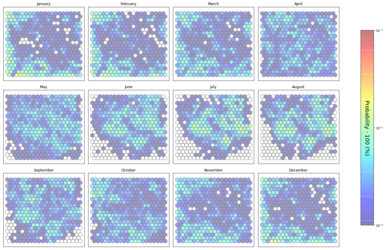
slopes_som = Slopes_SOM(data, beach='farolillo')
som, data_mean, data_count = slopes_som.train(som_shape=(20,20), sigma=0.8, learning_rate=0.5,
                                              num_iteration=50000, plot_results=False)
slopes_som.plot_results(som, data_mean, data_count, second_plot='Hb_index', plot_months=True)
The following data will be trained in: farolillo


The sum off all probabilities is: 1.0
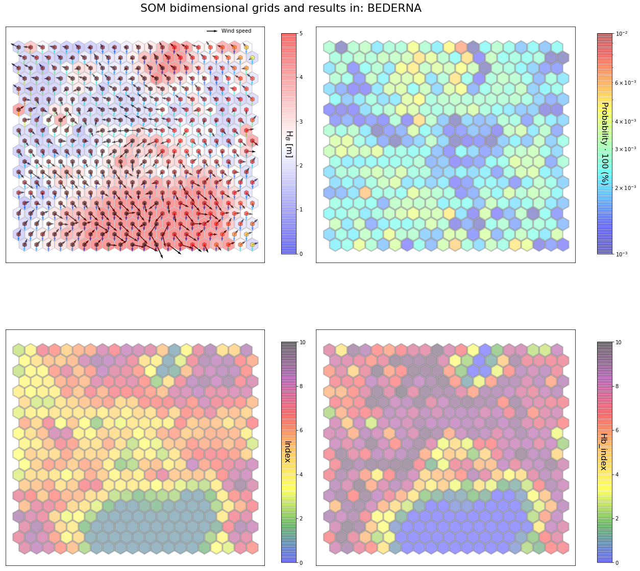
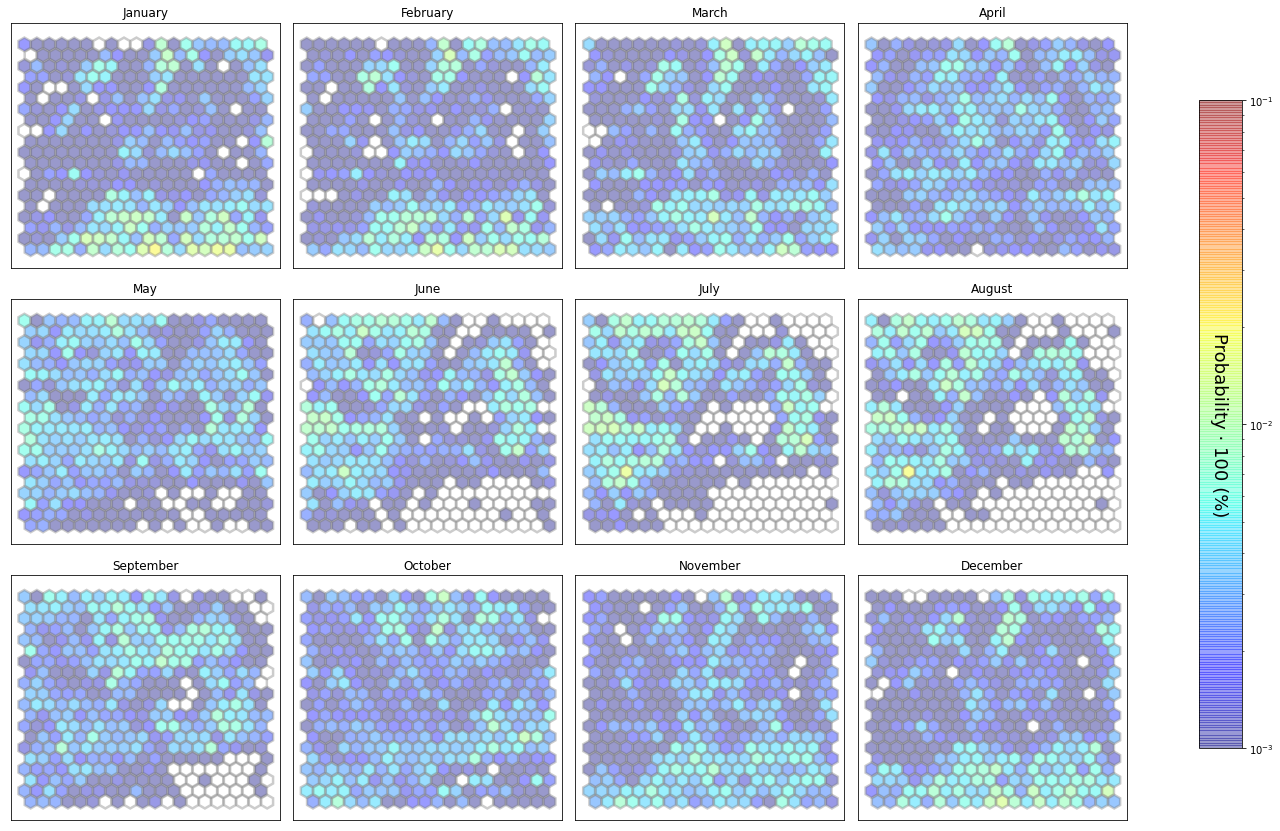
slopes_som = Slopes_SOM(data, beach='bederna')
som, data_mean, data_count = slopes_som.train(som_shape=(20,20), sigma=0.8, learning_rate=0.5,
                                              num_iteration=50000, plot_results=False)
slopes_som.plot_results(som, data_mean, data_count, second_plot='Hb_index', plot_months=True)
The following data will be trained in: bederna


The sum off all probabilities is: 1.0
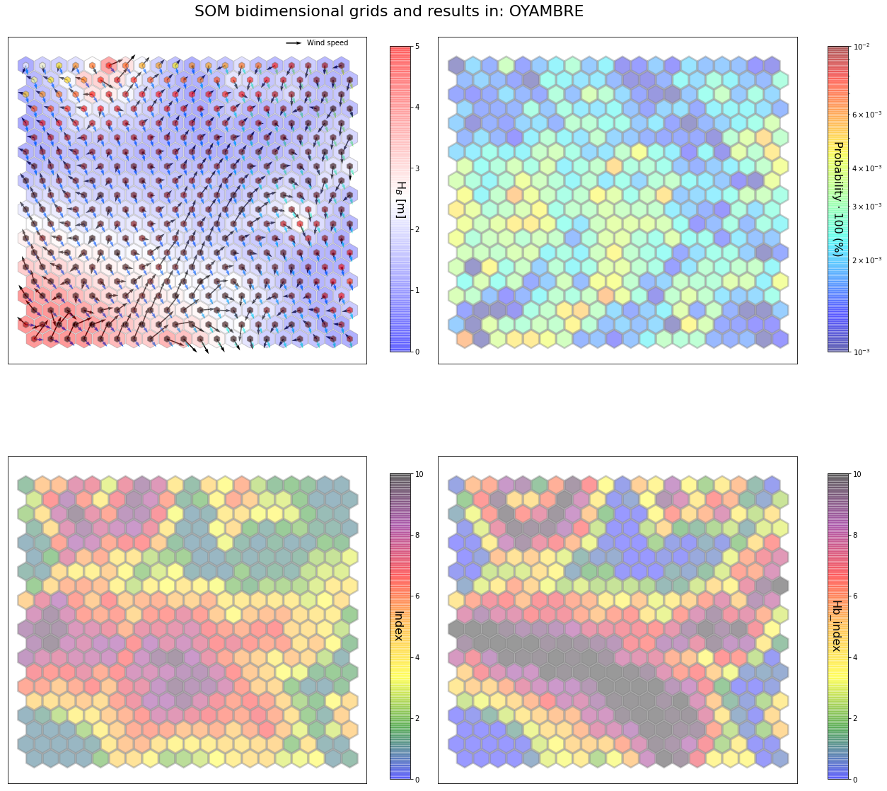
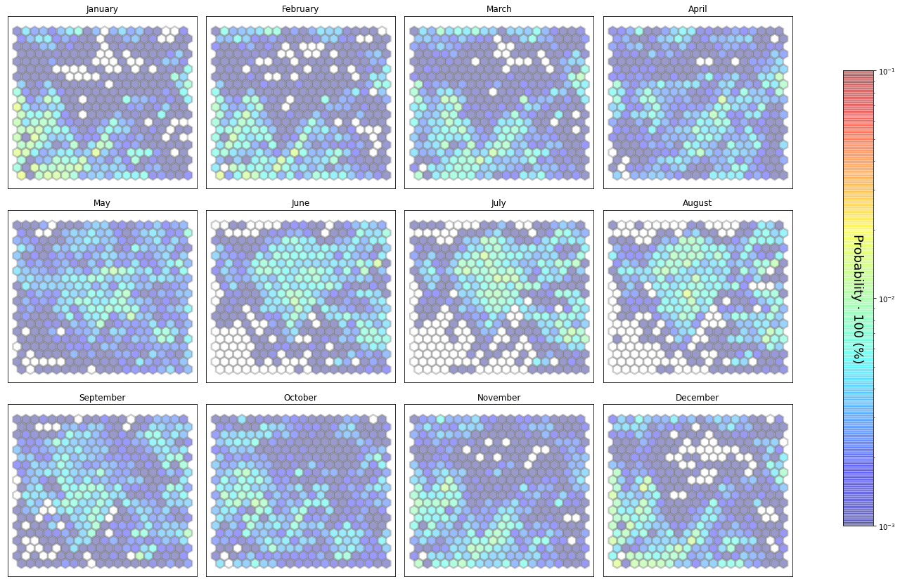
slopes_som = Slopes_SOM(data, beach='oyambre')
som, data_mean, data_count = slopes_som.train(som_shape=(20,20), sigma=0.8, learning_rate=0.5,
                                              num_iteration=50000, plot_results=False)
slopes_som.plot_results(som, data_mean, data_count, second_plot='Hb_index', plot_months=True)
The following data will be trained in: oyambre


The sum off all probabilities is: 1.0
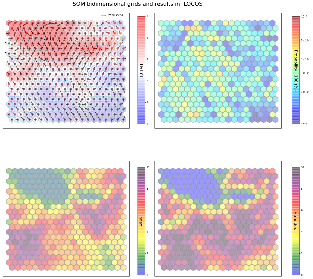
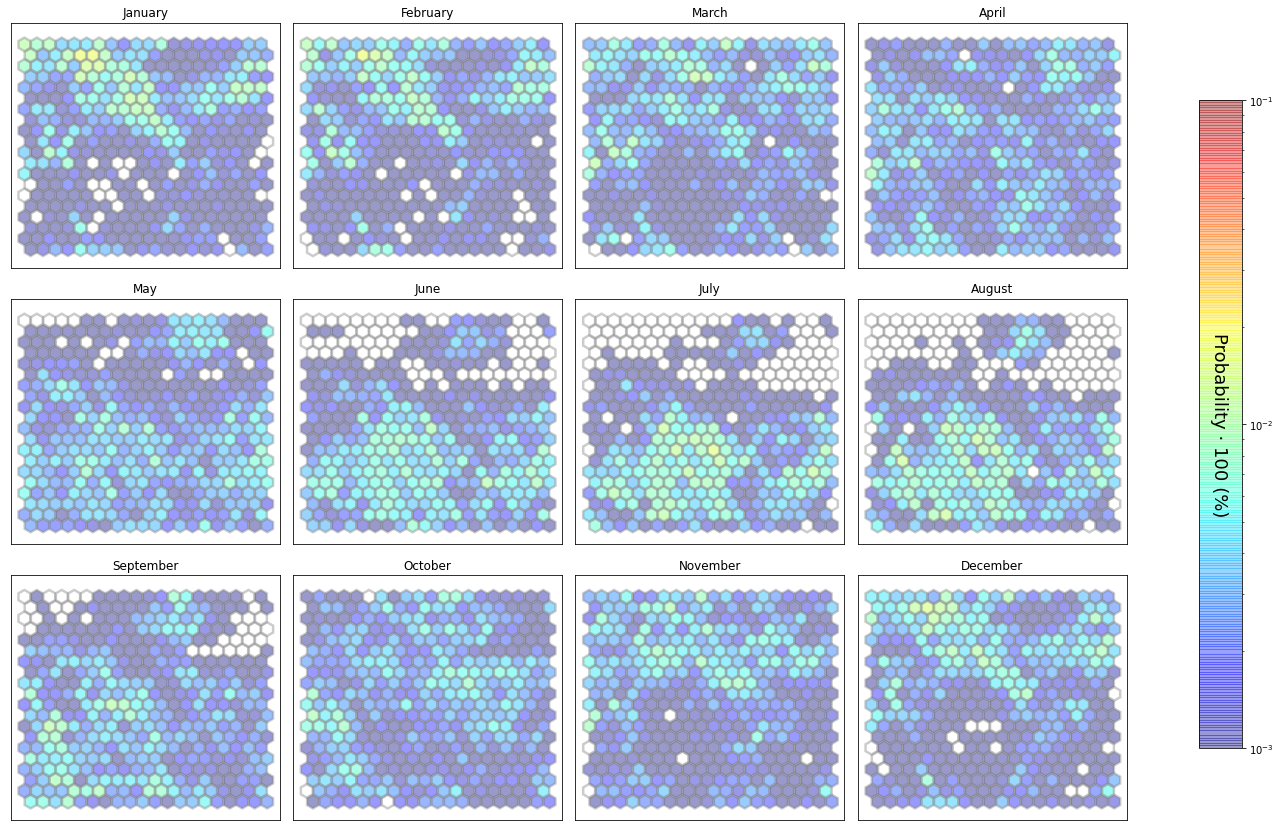
slopes_som = Slopes_SOM(data, beach='locos')
som, data_mean, data_count = slopes_som.train(som_shape=(20,20), sigma=0.8, learning_rate=0.5,
                                              num_iteration=50000, plot_results=False)
slopes_som.plot_results(som, data_mean, data_count, second_plot='Hb_index', plot_months=True)
The following data will be trained in: locos


The sum off all probabilities is: 0.9999999999999999
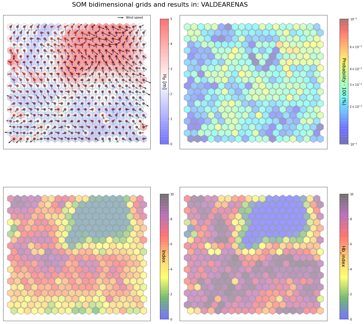
slopes_som = Slopes_SOM(data, beach='valdearenas')
som, data_mean, data_count = slopes_som.train(som_shape=(20,20), sigma=0.8, learning_rate=0.5,
                                              num_iteration=50000, plot_results=False)
slopes_som.plot_results(som, data_mean, data_count, second_plot='Hb_index', plot_months=True)
The following data will be trained in: valdearenas


The sum off all probabilities is: 1.0

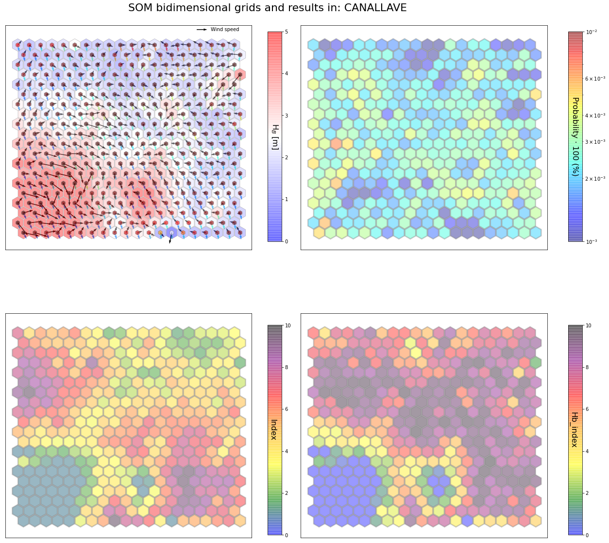
slopes_som = Slopes_SOM(data, beach='canallave')
som, data_mean, data_count = slopes_som.train(som_shape=(20,20), sigma=0.8, learning_rate=0.5,
                                              num_iteration=50000, plot_results=False)
slopes_som.plot_results(som, data_mean, data_count, second_plot='Hb_index', plot_months=True)
The following data will be trained in: canallave


The sum off all probabilities is: 1.0
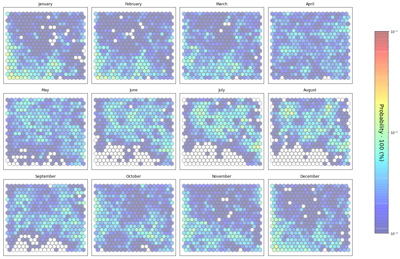
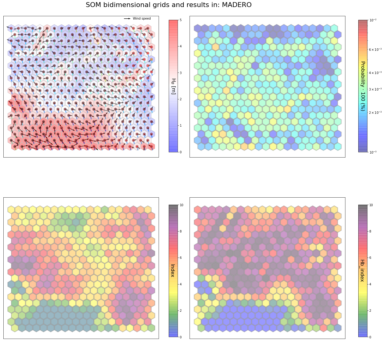
slopes_som = Slopes_SOM(data, beach='madero')
som, data_mean, data_count = slopes_som.train(som_shape=(20,20), sigma=0.8, learning_rate=0.5,
                                              num_iteration=50000, plot_results=False)
slopes_som.plot_results(som, data_mean, data_count, second_plot='Hb_index', plot_months=True)
The following data will be trained in: madero


The sum off all probabilities is: 1.0
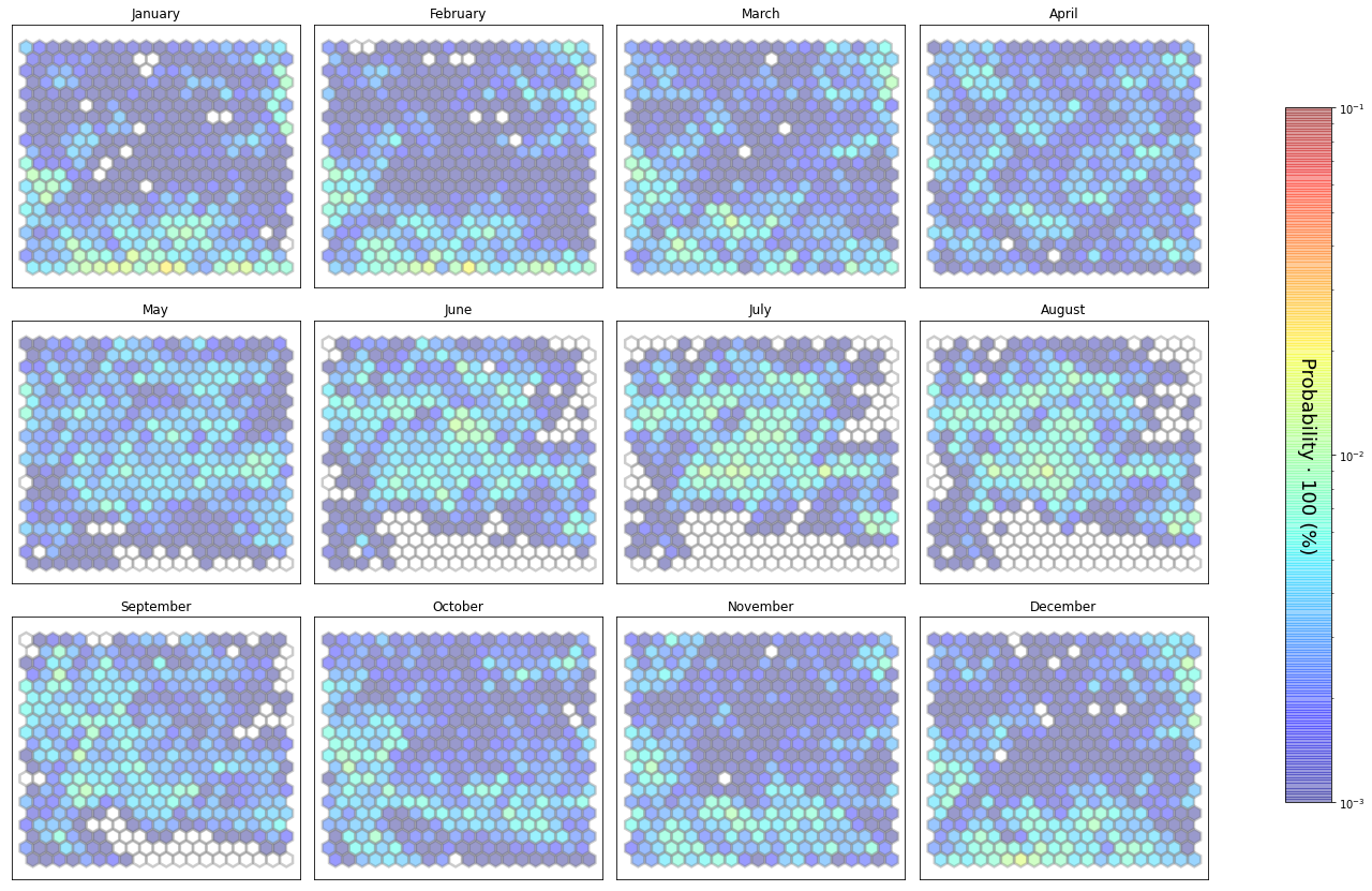
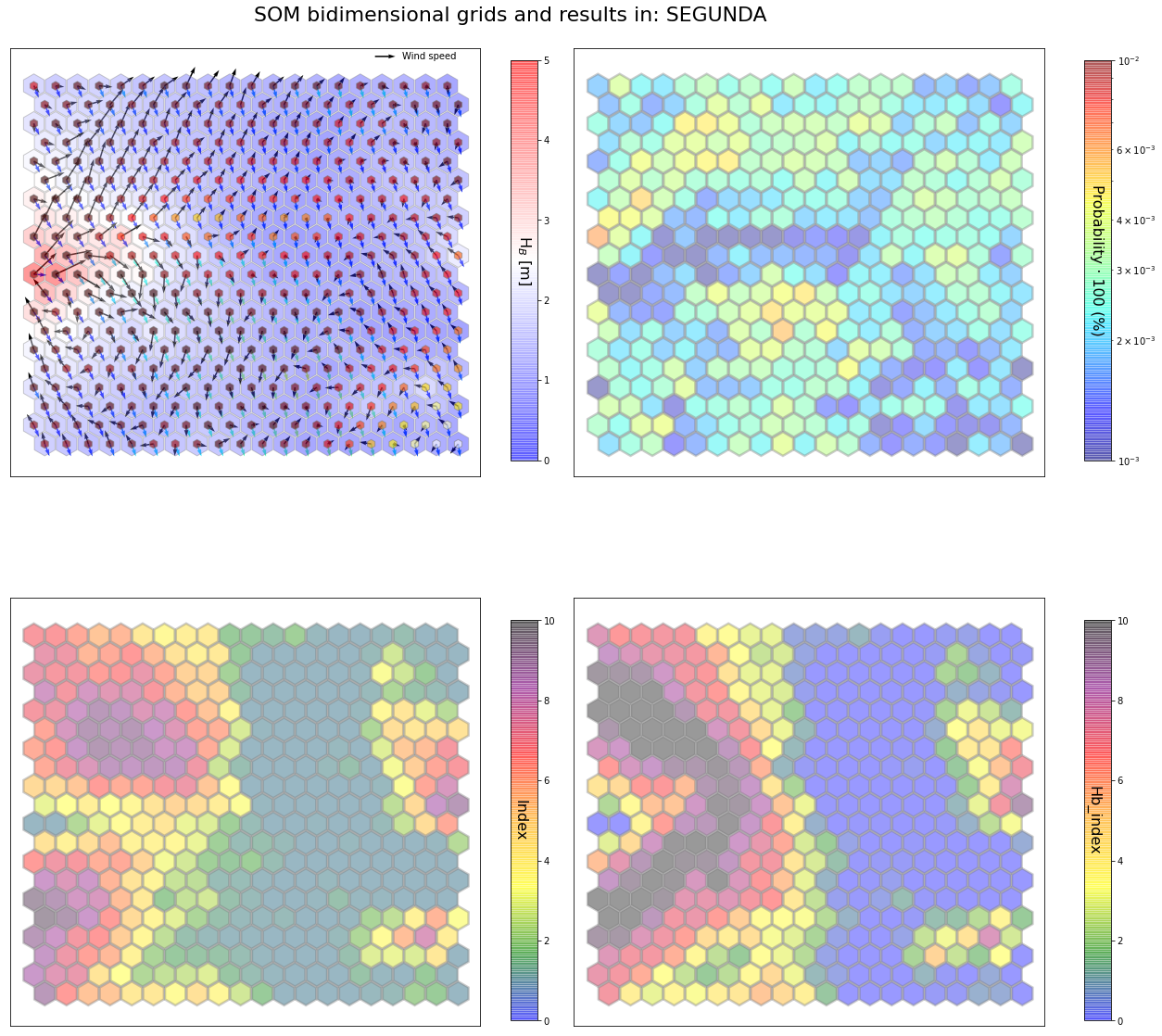
slopes_som = Slopes_SOM(data, beach='segunda')
som, data_mean, data_count = slopes_som.train(som_shape=(20,20), sigma=0.8, learning_rate=0.5,
                                              num_iteration=50000, plot_results=False)
slopes_som.plot_results(som, data_mean, data_count, second_plot='Hb_index', plot_months=True)
The following data will be trained in: segunda


The sum off all probabilities is: 1.0
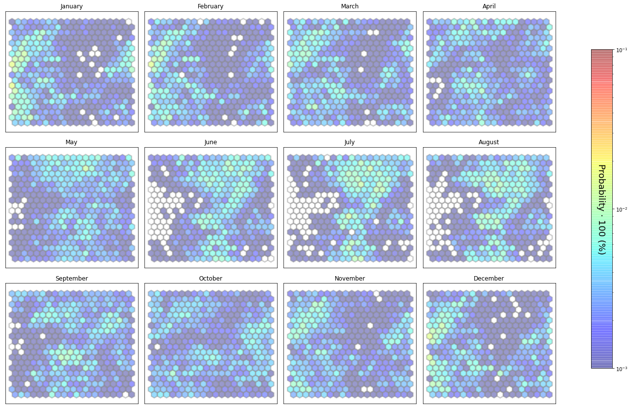
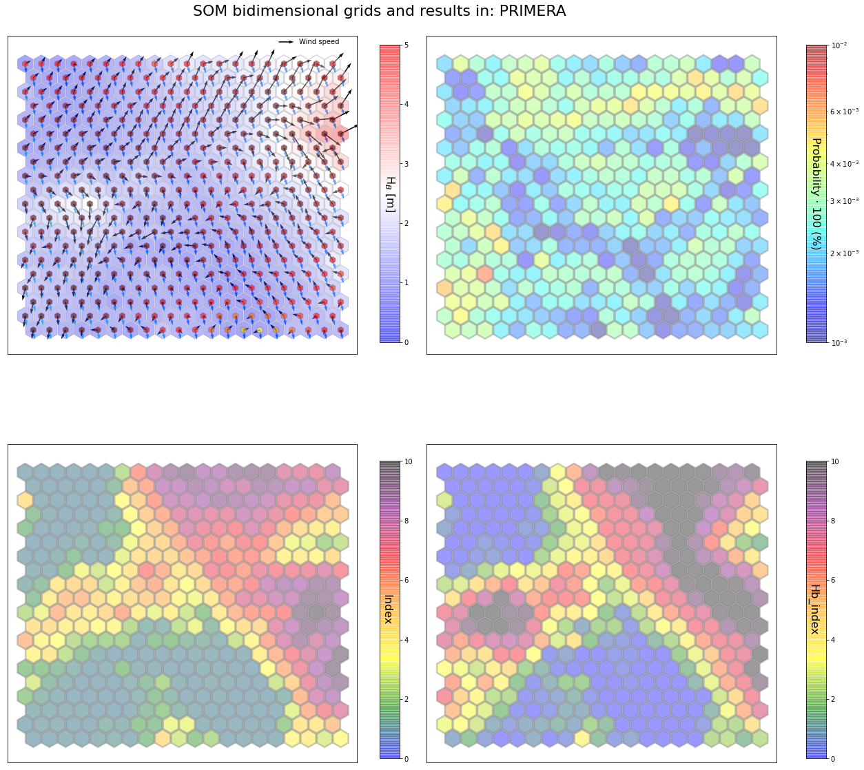
slopes_som = Slopes_SOM(data, beach='primera')
som, data_mean, data_count = slopes_som.train(som_shape=(20,20), sigma=0.8, learning_rate=0.5,
                                              num_iteration=50000, plot_results=False)
slopes_som.plot_results(som, data_mean, data_count, second_plot='Hb_index', plot_months=True)
The following data will be trained in: primera


The sum off all probabilities is: 1.0
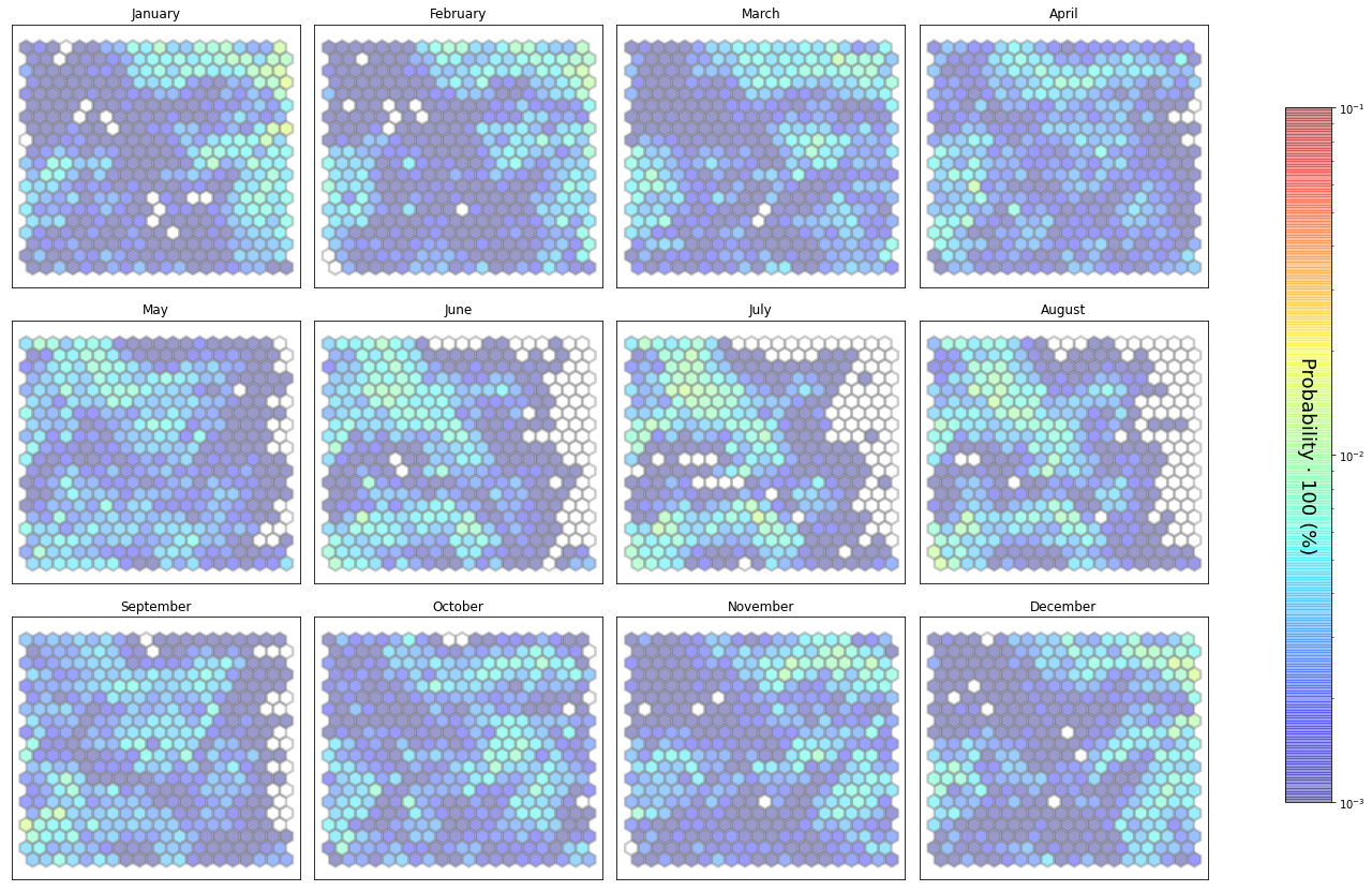
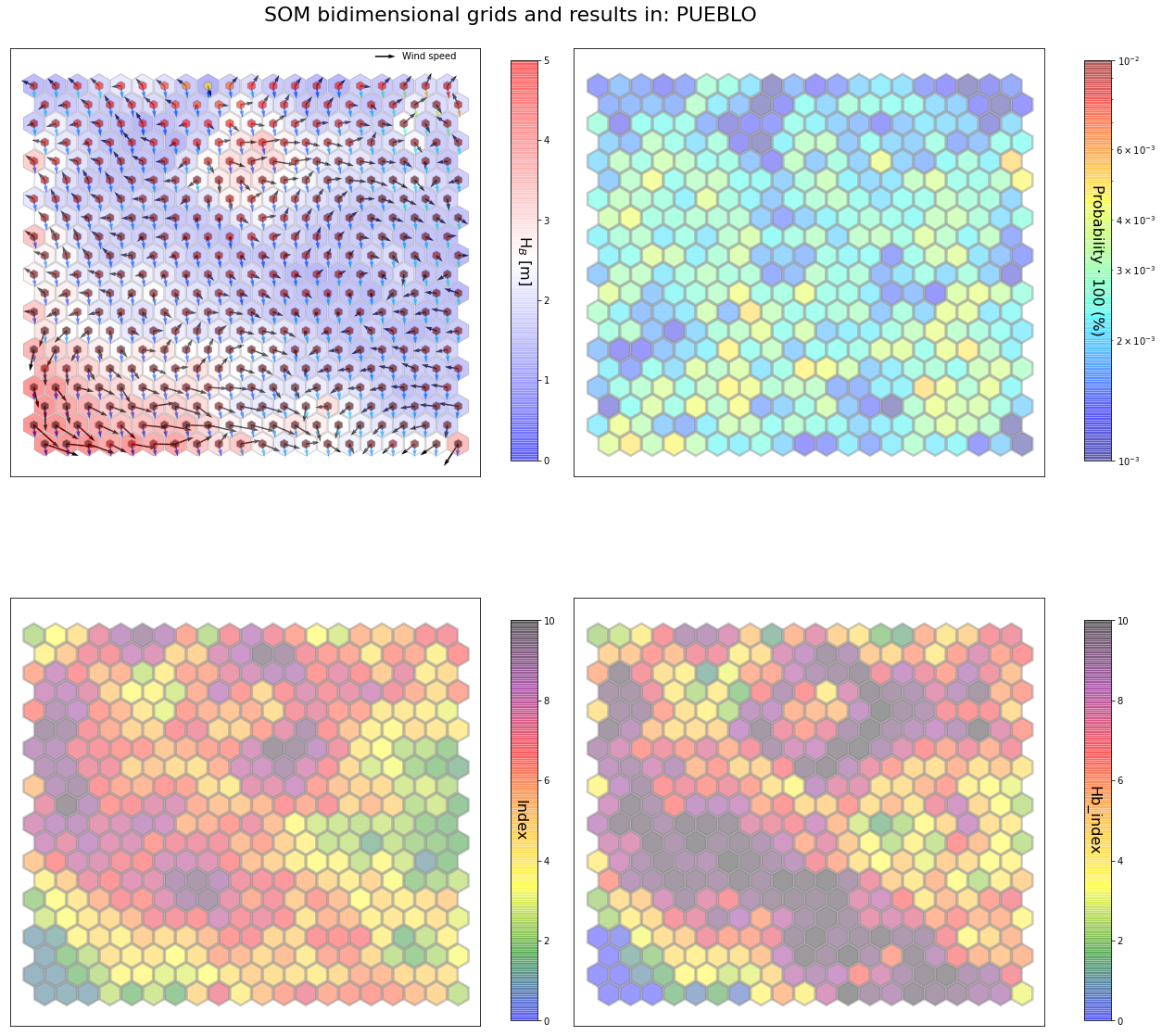
slopes_som = Slopes_SOM(data, beach='pueblo')
som, data_mean, data_count = slopes_som.train(som_shape=(20,20), sigma=0.8, learning_rate=0.5,
                                              num_iteration=50000, plot_results=False)
slopes_som.plot_results(som, data_mean, data_count, second_plot='Hb_index', plot_months=True)
The following data will be trained in: pueblo


The sum off all probabilities is: 1.0
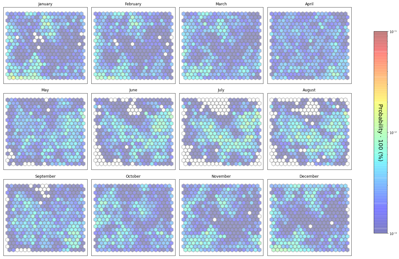
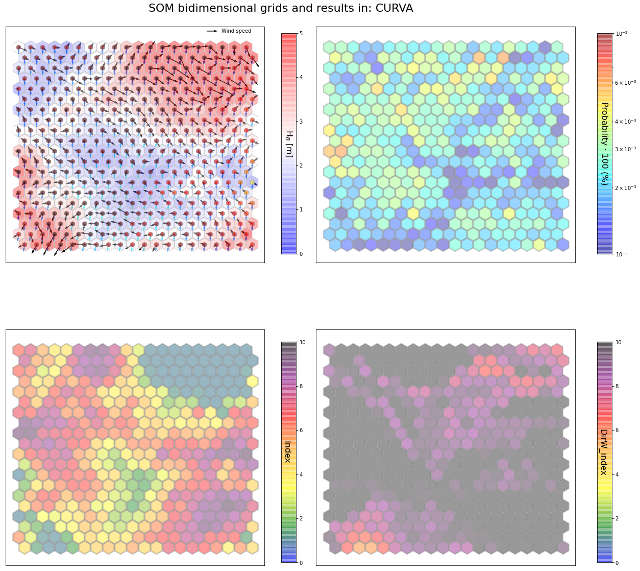
slopes_som = Slopes_SOM(data, beach='curva')
som, data_mean, data_count = slopes_som.train(som_shape=(20,20), sigma=0.8, learning_rate=0.5,
                                              num_iteration=50000, plot_results=False)
slopes_som.plot_results(som, data_mean, data_count, second_plot='DirW_index', plot_months=True)
The following data will be trained in: curva


The sum off all probabilities is: 1.0
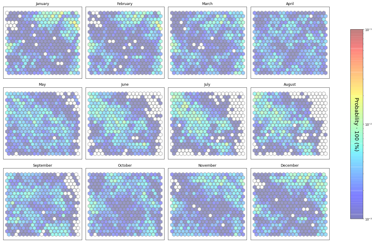
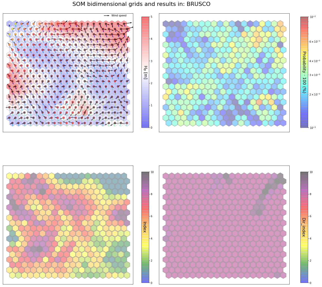
slopes_som = Slopes_SOM(data, beach='brusco')
som, data_mean, data_count = slopes_som.train(som_shape=(20,20), sigma=0.8, learning_rate=0.5,
                                              num_iteration=50000, plot_results=False)
slopes_som.plot_results(som, data_mean, data_count, second_plot='Dir_index', plot_months=True)
The following data will be trained in: brusco


The sum off all probabilities is: 1.0
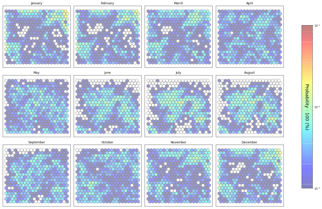
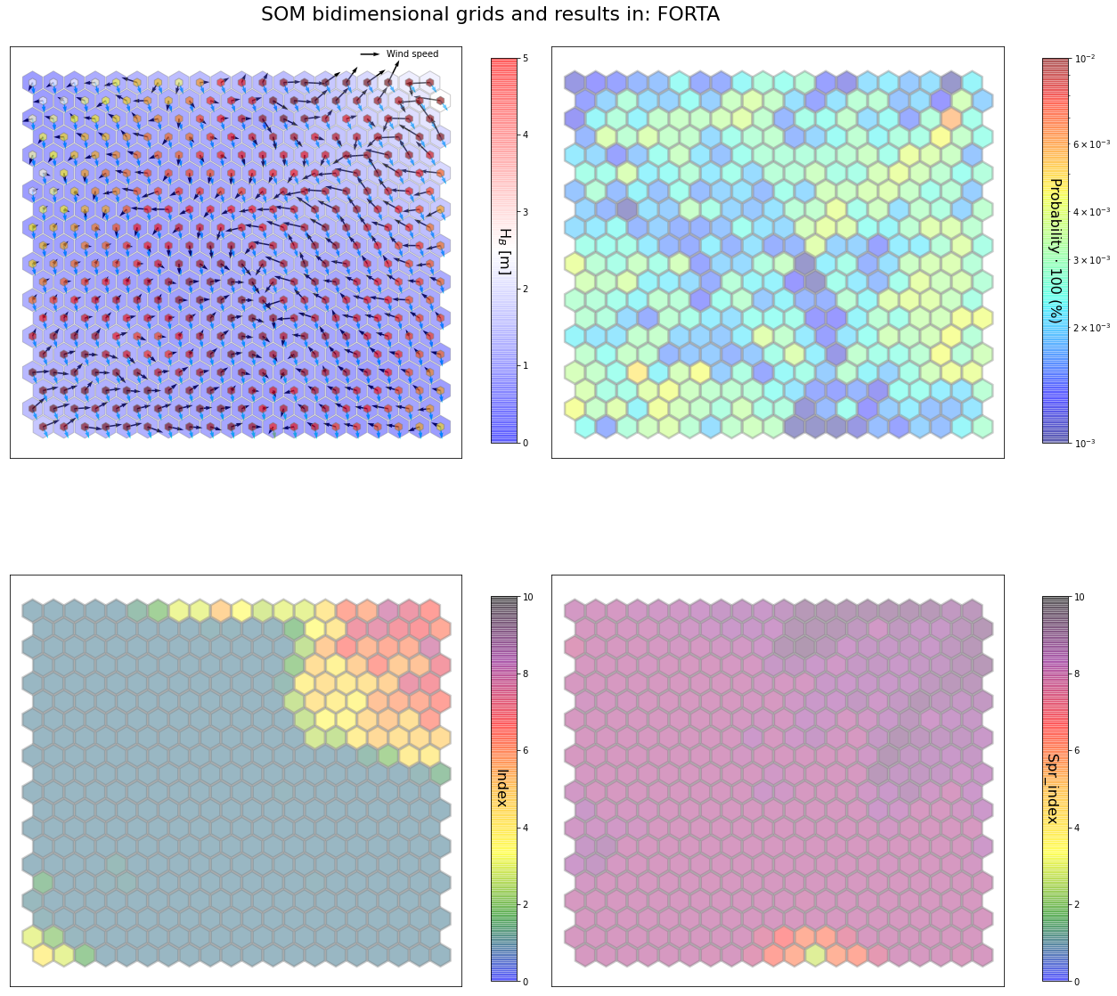
slopes_som = Slopes_SOM(data, beach='forta')
som, data_mean, data_count = slopes_som.train(som_shape=(20,20), sigma=0.8, learning_rate=0.5,
                                              num_iteration=50000, plot_results=False)
slopes_som.plot_results(som, data_mean, data_count, second_plot='Spr_index', plot_months=True)
The following data will be trained in: forta


The sum off all probabilities is: 1.0
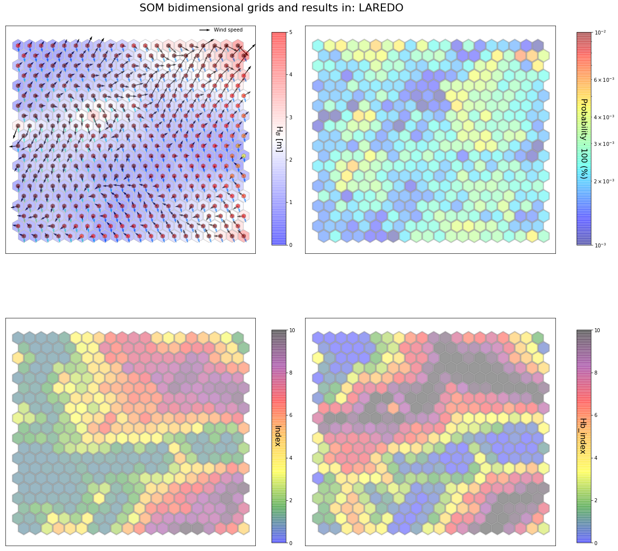
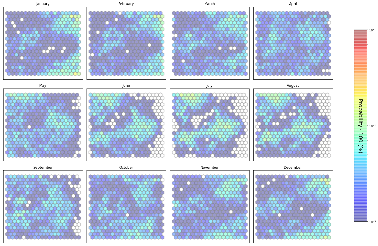
slopes_som = Slopes_SOM(data, beach='laredo')
som, data_mean, data_count = slopes_som.train(som_shape=(20,20), sigma=0.8, learning_rate=0.5,
                                              num_iteration=50000, plot_results=False)
slopes_som.plot_results(som, data_mean, data_count, second_plot='Hb_index', plot_months=True)
The following data will be trained in: laredo


The sum off all probabilities is: 1.0